---
title: "Chapter 15: 迴歸分析"
---
```{r}
#| include: false
source(here::here("R/_common.R"))
```
## 學習目標 {.unnumbered}
- 用微積分推導 OLS 迴歸係數
- 理解偏微分在多元迴歸中的角色
- 掌握 Logistic regression 的 log-odds 與微分
- 視覺化殘差平方和的 3D 曲面
- 連結 MLE 與迴歸分析
## 概念說明
### 迴歸分析是什麼?
迴歸分析是**用一個或多個變數(X)來預測另一個變數(Y)**的統計方法[@hastie2009elements]。
**醫學例子**:
- 用年齡、BMI 預測血壓
- 用腫瘤大小、淋巴結轉移預測存活時間
- 用劑量預測藥物反應
### 為什麼需要微積分?
迴歸的核心問題是**找到最佳的係數**,使得「預測值」與「實際值」的差距最小。這是一個**最佳化問題**,需要用微分來解。
## 簡單線性迴歸
### 模型
$$
y_i = \beta_0 + \beta_1 x_i + \varepsilon_i
$$
其中 $\varepsilon_i \sim N(0, \sigma^2)$ 是誤差項。
**目標**:找到 $\hat{\beta}_0, \hat{\beta}_1$ 使得預測最準確。
### 最小平方法 (OLS)
**殘差 (Residual)**:
$$
e_i = y_i - (\beta_0 + \beta_1 x_i)
$$
**殘差平方和 (RSS, Residual Sum of Squares)**:
$$
\text{RSS}(\beta_0, \beta_1) = \sum_{i=1}^{n} e_i^2 = \sum_{i=1}^{n} [y_i - (\beta_0 + \beta_1 x_i)]^2
$$
**目標**:最小化 RSS
$$
(\hat{\beta}_0, \hat{\beta}_1) = \arg\min_{\beta_0, \beta_1} \text{RSS}(\beta_0, \beta_1)
$$
## 視覺化理解
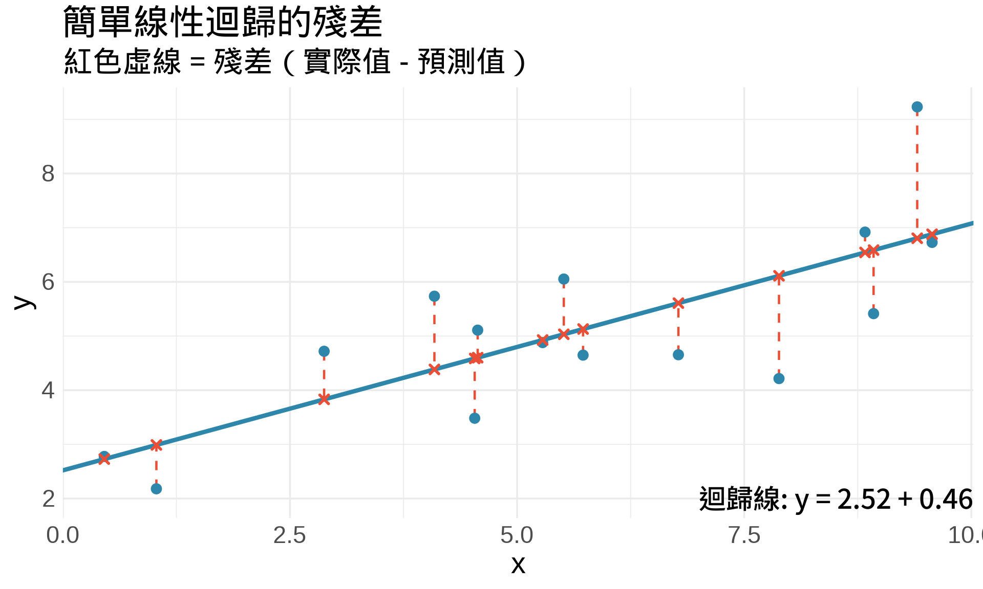
### 殘差的幾何意義
```{r}
#| label: fig-residuals
#| fig-cap: "殘差是「實際值」與「預測值」的垂直距離"
#| fig-width: 10
#| fig-height: 6
# 模擬資料
set.seed(123)
n <- 15
x <- runif(n, 0, 10)
y <- 2 + 0.5 * x + rnorm(n, 0, 1)

# 擬合迴歸
fit <- lm(y ~ x)
y_pred <- fitted(fit)

df <- data.frame(x, y, y_pred)

ggplot(df, aes(x, y)) +
  # 殘差線段
  geom_segment(aes(xend = x, yend = y_pred),
               color = "#E94F37", linetype = "dashed", linewidth = 0.8) +
  # 迴歸線
  geom_abline(intercept = coef(fit)[1], slope = coef(fit)[2],
              color = "#2E86AB", linewidth = 1.5) +
  # 觀察點
  geom_point(size = 3, color = "#2E86AB") +
  # 預測點
  geom_point(aes(y = y_pred), size = 2, color = "#E94F37", shape = 4, stroke = 1.5) +
  annotate("text", x = 7, y = 2,
           label = paste0("迴歸線: y = ", round(coef(fit)[1], 2),
                         " + ", round(coef(fit)[2], 2), "x"),
           size = 4.5, hjust = 0) +
  labs(
    title = "簡單線性迴歸的殘差",
    subtitle = "紅色虛線 = 殘差(實際值 - 預測值)",
    x = "x", y = "y"
  ) +
  theme_minimal(base_size = 14)
```
### 殘差平方和的 3D 曲面
```{r}
#| label: fig-rss-surface
#| fig-cap: "RSS 是一個碗狀的 3D 曲面"
#| fig-width: 10
#| fig-height: 8
library(plotly)

# 建立 RSS 函數
rss <- function(beta0, beta1) {
  y_pred <- beta0 + beta1 * x
  sum((y - y_pred)^2)
}

# 建立網格
beta0_seq <- seq(0, 4, length.out = 50)
beta1_seq <- seq(-0.5, 1.5, length.out = 50)

rss_grid <- outer(beta0_seq, beta1_seq, Vectorize(rss))

# OLS 估計值
beta0_hat <- coef(fit)[1]
beta1_hat <- coef(fit)[2]

plot_ly(x = beta0_seq, y = beta1_seq, z = rss_grid,
        type = "surface",
        colorscale = list(c(0, "#2E86AB"), c(1, "#E94F37"))) %>%
  add_trace(x = beta0_hat, y = beta1_hat,
            z = rss(beta0_hat, beta1_hat),
            type = "scatter3d", mode = "markers",
            marker = list(size = 8, color = "yellow"),
            name = "OLS 估計值") %>%
  layout(
    title = "殘差平方和 (RSS) 的 3D 曲面",
    scene = list(
      xaxis = list(title = "β₀ (截距)"),
      yaxis = list(title = "β₁ (斜率)"),
      zaxis = list(title = "RSS")
    )
  )
```
**關鍵洞察**:
- RSS 是一個**凸函數**(碗狀),有唯一最小值
- 最小值位置 = OLS 估計值
- 用微分找最小值
## 數學推導
### OLS 估計值的微積分推導
**目標函數**:
$$
\text{RSS}(\beta_0, \beta_1) = \sum_{i=1}^{n} [y_i - \beta_0 - \beta_1 x_i]^2
$$
**對 $\beta_0$ 偏微分**:
$$
\frac{\partial \text{RSS}}{\partial \beta_0} = -2\sum_{i=1}^{n}(y_i - \beta_0 - \beta_1 x_i) = 0
$$
$$
\Rightarrow n\beta_0 + \beta_1\sum_{i=1}^{n}x_i = \sum_{i=1}^{n}y_i
$$
$$
\Rightarrow \beta_0 = \bar{y} - \beta_1\bar{x} \quad \text{...(1)}
$$
**對 $\beta_1$ 偏微分**:
$$
\frac{\partial \text{RSS}}{\partial \beta_1} = -2\sum_{i=1}^{n}x_i(y_i - \beta_0 - \beta_1 x_i) = 0
$$
將 (1) 代入:
$$
\sum_{i=1}^{n}x_i[y_i - (\bar{y} - \beta_1\bar{x}) - \beta_1 x_i] = 0
$$
$$
\sum_{i=1}^{n}x_i(y_i - \bar{y}) = \beta_1\sum_{i=1}^{n}x_i(x_i - \bar{x})
$$
$$
\Rightarrow \boxed{\hat{\beta}_1 = \frac{\sum_{i=1}^{n}(x_i - \bar{x})(y_i - \bar{y})}{\sum_{i=1}^{n}(x_i - \bar{x})^2} = \frac{\text{Cov}(x, y)}{\text{Var}(x)}}
$$
$$
\boxed{\hat{\beta}_0 = \bar{y} - \hat{\beta}_1\bar{x}}
$$
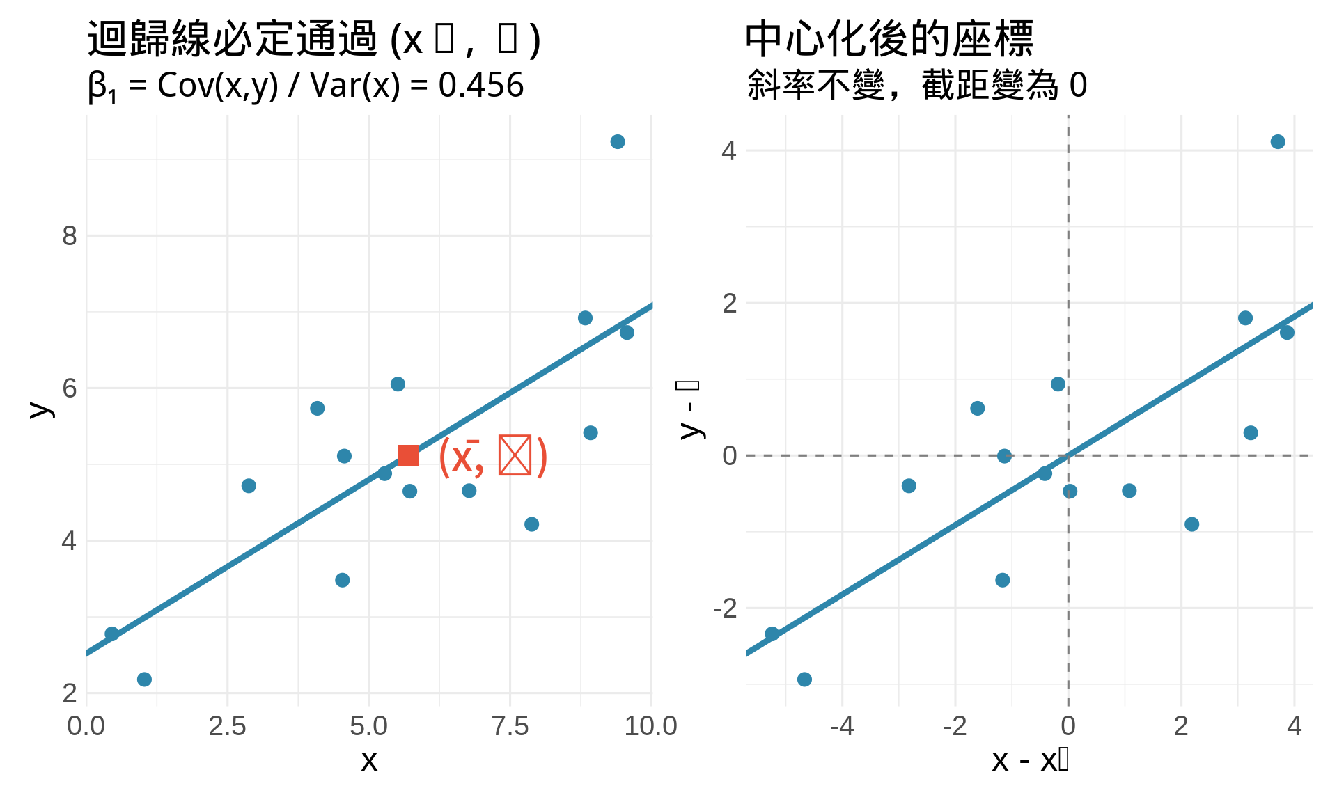
### 視覺化推導過程
```{r}
#| label: fig-ols-derivation
#| fig-cap: "OLS 估計值的幾何意義"
#| fig-width: 10
#| fig-height: 6
# 計算 OLS 估計值
x_bar <- mean(x)
y_bar <- mean(y)
beta1_hat <- sum((x - x_bar) * (y - y_bar)) / sum((x - x_bar)^2)
beta0_hat <- y_bar - beta1_hat * x_bar

p1 <- ggplot(data.frame(x, y), aes(x, y)) +
  geom_point(size = 3, color = "#2E86AB") +
  geom_abline(intercept = beta0_hat, slope = beta1_hat,
              color = "#2E86AB", linewidth = 1.5) +
  # 平均數點
  geom_point(aes(x = x_bar, y = y_bar),
             color = "#E94F37", size = 5, shape = 15) +
  annotate("text", x = x_bar + 0.5, y = y_bar,
           label = paste0("(x̄, ȳ)"),
           size = 5, hjust = 0, color = "#E94F37") +
  labs(
    title = "迴歸線必定通過 (x̄, ȳ)",
    subtitle = paste0("β₁ = Cov(x,y) / Var(x) = ", round(beta1_hat, 3)),
    x = "x", y = "y"
  ) +
  theme_minimal(base_size = 12)

# 標準化座標
x_centered <- x - x_bar
y_centered <- y - y_bar

p2 <- ggplot(data.frame(x_centered, y_centered),
             aes(x_centered, y_centered)) +
  geom_point(size = 3, color = "#2E86AB") +
  geom_abline(intercept = 0, slope = beta1_hat,
              color = "#2E86AB", linewidth = 1.5) +
  geom_vline(xintercept = 0, linetype = "dashed", color = "gray50") +
  geom_hline(yintercept = 0, linetype = "dashed", color = "gray50") +
  labs(
    title = "中心化後的座標",
    subtitle = "斜率不變,截距變為 0",
    x = "x - x̄", y = "y - ȳ"
  ) +
  theme_minimal(base_size = 12)

p1 + p2
```
## 多元線性迴歸
### 模型
$$
y_i = \beta_0 + \beta_1 x_{i1} + \beta_2 x_{i2} + \cdots + \beta_p x_{ip} + \varepsilon_i
$$
**矩陣形式**:
$$
\mathbf{y} = \mathbf{X}\boldsymbol{\beta} + \boldsymbol{\varepsilon}
$$
### 矩陣推導
**RSS**:
$$
\text{RSS}(\boldsymbol{\beta}) = (\mathbf{y} - \mathbf{X}\boldsymbol{\beta})^T(\mathbf{y} - \mathbf{X}\boldsymbol{\beta})
$$
**對 $\boldsymbol{\beta}$ 微分**(用向量微積分):
$$
\frac{\partial \text{RSS}}{\partial \boldsymbol{\beta}} = -2\mathbf{X}^T(\mathbf{y} - \mathbf{X}\boldsymbol{\beta}) = \mathbf{0}
$$
$$
\Rightarrow \mathbf{X}^T\mathbf{X}\boldsymbol{\beta} = \mathbf{X}^T\mathbf{y}
$$
$$
\Rightarrow \boxed{\hat{\boldsymbol{\beta}} = (\mathbf{X}^T\mathbf{X})^{-1}\mathbf{X}^T\mathbf{y}}
$$
這就是著名的 **Normal Equation**。
```{r}
#| label: fig-multiple-regression
#| fig-cap: "多元迴歸:預測血壓"
#| fig-width: 10
#| fig-height: 8
# 模擬資料:血壓 ~ 年齡 + BMI
set.seed(456)
n <- 100
age <- runif(n, 30, 70)
bmi <- runif(n, 18, 35)
bp <- 80 + 0.5 * age + 1.2 * bmi + rnorm(n, 0, 5)

# 擬合多元迴歸
fit_multi <- lm(bp ~ age + bmi)

# 3D 散點圖與迴歸平面
library(plotly)

# 建立預測網格
age_seq <- seq(30, 70, length.out = 30)
bmi_seq <- seq(18, 35, length.out = 30)
grid <- expand.grid(age = age_seq, bmi = bmi_seq)
grid$bp_pred <- predict(fit_multi, newdata = grid)

bp_matrix <- matrix(grid$bp_pred, nrow = 30, ncol = 30)

plot_ly() %>%
  add_trace(x = age, y = bmi, z = bp,
            type = "scatter3d", mode = "markers",
            marker = list(size = 3, color = "#2E86AB"),
            name = "觀察資料") %>%
  add_surface(x = age_seq, y = bmi_seq, z = bp_matrix,
              opacity = 0.7,
              colorscale = list(c(0, "#E94F37"), c(1, "#6A994E")),
              name = "迴歸平面") %>%
  layout(
    title = "多元迴歸:血壓 ~ 年齡 + BMI",
    scene = list(
      xaxis = list(title = "年齡"),
      yaxis = list(title = "BMI"),
      zaxis = list(title = "血壓")
    )
  )
```
## Logistic Regression
### 模型
用於**二元結果**(如疾病有無、存活與否):
$$
\log\left(\frac{p_i}{1-p_i}\right) = \beta_0 + \beta_1 x_i
$$
其中 $p_i = P(Y_i = 1 | x_i)$
**解出 $p_i$**:
$$
p_i = \frac{e^{\beta_0 + \beta_1 x_i}}{1 + e^{\beta_0 + \beta_1 x_i}} = \frac{1}{1 + e^{-(\beta_0 + \beta_1 x_i)}}
$$
### Log-Odds 的微分
**Odds**:
$$
\text{Odds} = \frac{p}{1-p}
$$
**Log-Odds (Logit)**:
$$
\text{Logit}(p) = \log\left(\frac{p}{1-p}\right)
$$
**微分**:
$$
\frac{d}{dp}\text{Logit}(p) = \frac{d}{dp}\log\left(\frac{p}{1-p}\right) = \frac{1}{p(1-p)}
$$
這說明:**當 $p$ 接近 0 或 1 時,log-odds 的變化率很大**。
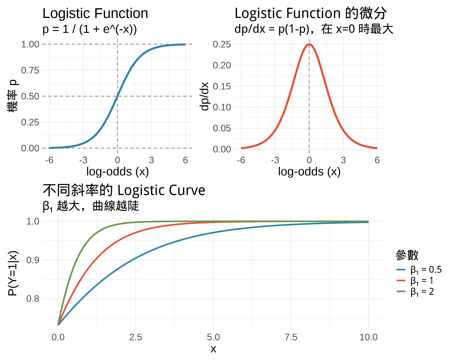
### 視覺化 Logistic Function
```{r}
#| label: fig-logistic-function
#| fig-cap: "Logistic function:從 log-odds 到機率"
#| fig-width: 10
#| fig-height: 8
# Logit 和 逆 Logit
x <- seq(-6, 6, by = 0.01)
logit_to_prob <- function(x) 1 / (1 + exp(-x))

p1 <- ggplot(data.frame(x), aes(x)) +
  stat_function(fun = logit_to_prob,
                color = "#2E86AB", linewidth = 1.5) +
  geom_hline(yintercept = c(0, 0.5, 1),
             linetype = "dashed", color = "gray50") +
  geom_vline(xintercept = 0, linetype = "dashed", color = "gray50") +
  labs(
    title = "Logistic Function",
    subtitle = "p = 1 / (1 + e^(-x))",
    x = "log-odds (x)",
    y = "機率 p"
  ) +
  theme_minimal(base_size = 12)

# 微分:dp/dx
dlogistic <- function(x) {
  p <- logit_to_prob(x)
  p * (1 - p)
}

p2 <- ggplot(data.frame(x), aes(x)) +
  stat_function(fun = dlogistic,
                color = "#E94F37", linewidth = 1.5) +
  geom_vline(xintercept = 0, linetype = "dashed", color = "gray50") +
  labs(
    title = "Logistic Function 的微分",
    subtitle = "dp/dx = p(1-p),在 x=0 時最大",
    x = "log-odds (x)",
    y = "dp/dx"
  ) +
  theme_minimal(base_size = 12)

# Odds ratio 解釋
p3 <- ggplot(data.frame(x = c(0, 10)), aes(x)) +
  stat_function(fun = function(x) logit_to_prob(1 + 0.5*x),
                aes(color = "β₁ = 0.5"), linewidth = 1.2) +
  stat_function(fun = function(x) logit_to_prob(1 + 1*x),
                aes(color = "β₁ = 1"), linewidth = 1.2) +
  stat_function(fun = function(x) logit_to_prob(1 + 2*x),
                aes(color = "β₁ = 2"), linewidth = 1.2) +
  scale_color_manual(values = c("#2E86AB", "#E94F37", "#6A994E")) +
  labs(
    title = "不同斜率的 Logistic Curve",
    subtitle = "β₁ 越大,曲線越陡",
    x = "x",
    y = "P(Y=1|x)",
    color = "參數"
  ) +
  theme_minimal(base_size = 12)

(p1 + p2) / p3
```
### Logistic Regression 的 MLE
**Log-Likelihood**(見 Chapter 14):
$$
\ell(\beta_0, \beta_1) = \sum_{i=1}^{n}\left[y_i(\beta_0 + \beta_1 x_i) - \log(1 + e^{\beta_0 + \beta_1 x_i})\right]
$$
**Score Functions**:
$$
\frac{\partial \ell}{\partial\beta_0} = \sum_{i=1}^{n}(y_i - p_i) = 0
$$
$$
\frac{\partial \ell}{\partial\beta_1} = \sum_{i=1}^{n}x_i(y_i - p_i) = 0
$$
**解釋**:
- 殘差的加權和 = 0(權重是 $x_i$)
- 沒有解析解,需要數值方法(如 Newton-Raphson)
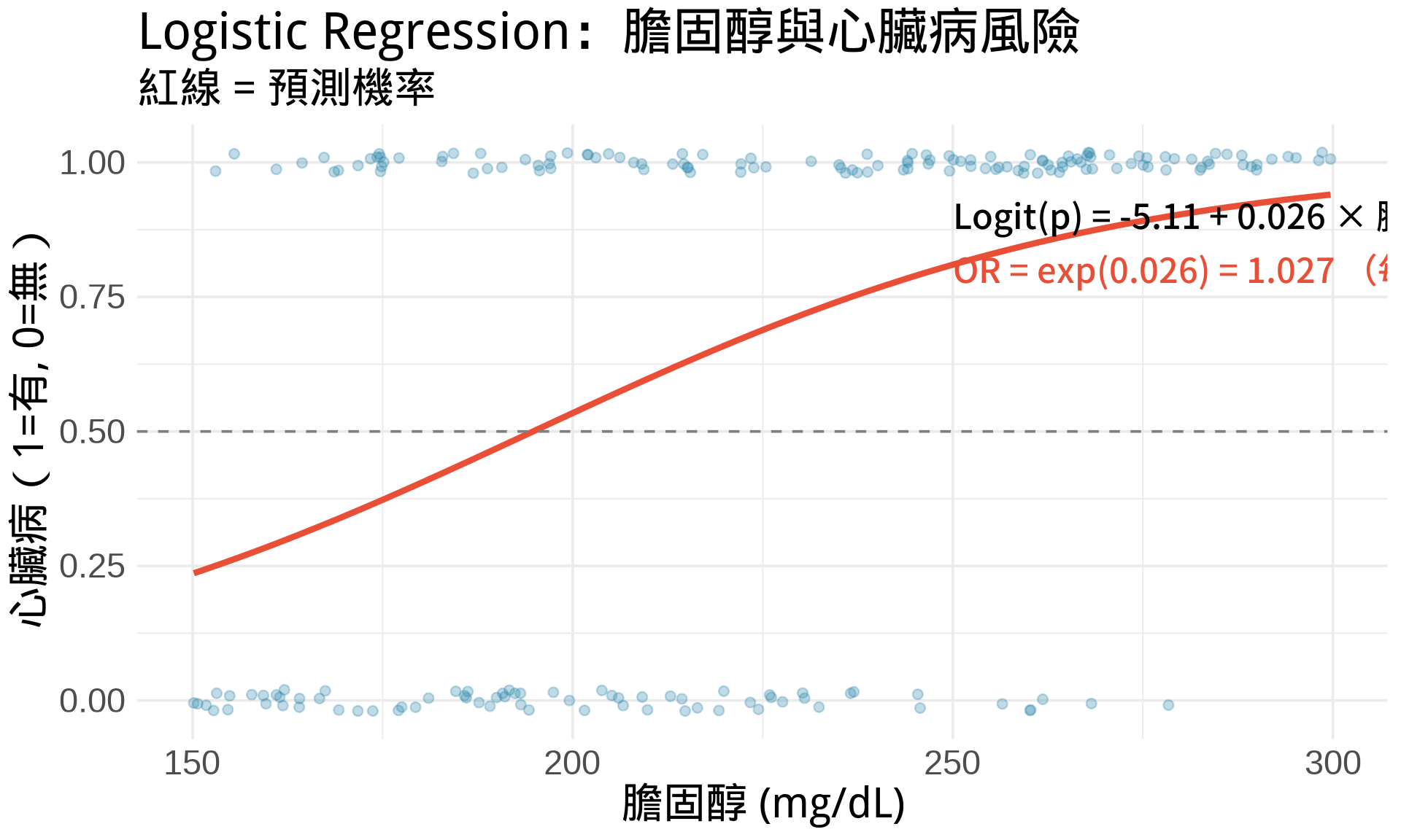
```{r}
#| label: fig-logistic-mle-example
#| fig-cap: "Logistic Regression 實例:預測心臟病風險"
#| fig-width: 10
#| fig-height: 6
# 模擬資料
set.seed(789)
n <- 200
cholesterol <- runif(n, 150, 300)
true_beta0 <- -8
true_beta1 <- 0.04

prob <- 1 / (1 + exp(-(true_beta0 + true_beta1 * cholesterol)))
heart_disease <- rbinom(n, 1, prob)

# 擬合 Logistic regression
fit_logistic <- glm(heart_disease ~ cholesterol, family = binomial)

df_logistic <- data.frame(
  cholesterol,
  heart_disease,
  prob_pred = fitted(fit_logistic)
)

ggplot(df_logistic, aes(cholesterol, heart_disease)) +
  geom_point(alpha = 0.3, size = 2,
             position = position_jitter(height = 0.02),
             color = "#2E86AB") +
  geom_line(aes(y = prob_pred), color = "#E94F37", linewidth = 1.5) +
  geom_hline(yintercept = 0.5, linetype = "dashed", color = "gray50") +
  annotate("text", x = 250, y = 0.9,
           label = paste0("Logit(p) = ", round(coef(fit_logistic)[1], 2),
                         " + ", round(coef(fit_logistic)[2], 3), " × 膽固醇"),
           size = 4, hjust = 0) +
  annotate("text", x = 250, y = 0.8,
           label = paste0("OR = exp(", round(coef(fit_logistic)[2], 3),
                         ") = ", round(exp(coef(fit_logistic)[2]), 3),
                         " (每增加 1 mg/dL)"),
           size = 4, hjust = 0, color = "#E94F37") +
  labs(
    title = "Logistic Regression:膽固醇與心臟病風險",
    subtitle = "紅線 = 預測機率",
    x = "膽固醇 (mg/dL)",
    y = "心臟病(1=有, 0=無)"
  ) +
  theme_minimal(base_size = 14)
```
## 練習題
### 觀念題
1. 為什麼 OLS 估計值一定通過 $(\bar{x}, \bar{y})$?
::: {.callout-tip collapse="true" title="參考答案"}
從數學推導可知 $\hat{\beta}_0 = \bar{y} - \hat{\beta}_1\bar{x}$。將 $(\bar{x}, \bar{y})$ 代入迴歸線方程式:$\hat{y} = \hat{\beta}_0 + \hat{\beta}_1\bar{x} = (\bar{y} - \hat{\beta}_1\bar{x}) + \hat{\beta}_1\bar{x} = \bar{y}$。這說明無論斜率為何,迴歸線必定通過資料的「中心點」$(\bar{x}, \bar{y})$。
:::
2. 在多元迴歸中,$\beta_1$ 的意義是什麼?(提示:「固定其他變數」)
::: {.callout-tip collapse="true" title="參考答案"}
$\beta_1$ 代表「在固定其他所有變數不變的情況下,$x_1$ 每增加 1 單位,$y$ 的平均變化量」。這就是偏微分的概念:$\beta_1 = \frac{\partial y}{\partial x_1}$。例如在血壓 ~ 年齡 + BMI 的模型中,年齡係數代表「同樣 BMI 的人,年齡每增加 1 歲,血壓平均增加多少」。
:::
3. 為什麼 Logistic regression 用 log-odds 而不是直接用機率?
::: {.callout-tip collapse="true" title="參考答案"}
機率 $p$ 被限制在 [0,1] 之間,無法直接做線性建模。但 log-odds $\log(p/(1-p))$ 的範圍是 $(-\infty, \infty)$,可以與自變數建立線性關係。此外,log-odds 的微分 $\frac{1}{p(1-p)}$ 在 $p$ 接近 0 或 1 時變化率很大,符合實際情境(效應在極端機率時更顯著)。
:::
### 計算題
1. 資料:$(x, y) = (1, 2), (2, 3), (3, 5)$。手算 OLS 估計值。
::: {.callout-tip collapse="true" title="參考答案"}
先算平均值:$\bar{x} = 2, \bar{y} = \frac{10}{3}$。計算 $\hat{\beta}_1 = \frac{\sum(x_i - \bar{x})(y_i - \bar{y})}{\sum(x_i - \bar{x})^2} = \frac{(-1)(-\frac{4}{3}) + 0 \cdot (-\frac{1}{3}) + 1 \cdot \frac{5}{3}}{1 + 0 + 1} = \frac{\frac{4}{3} + \frac{5}{3}}{2} = 1.5$。再算 $\hat{\beta}_0 = \bar{y} - \hat{\beta}_1\bar{x} = \frac{10}{3} - 1.5 \times 2 = \frac{1}{3} \approx 0.33$。迴歸方程式:$\hat{y} = 0.33 + 1.5x$。
:::
2. 已知 Logistic regression:$\text{Logit}(p) = -2 + 0.5x$。
- 當 $x = 4$ 時,$p = ?$
- Odds ratio = ?
::: {.callout-tip collapse="true" title="參考答案"}
當 $x = 4$ 時,$\text{Logit}(p) = -2 + 0.5 \times 4 = 0$,所以 $p = \frac{1}{1 + e^{0}} = 0.5$。Odds ratio = $\exp(\beta_1) = \exp(0.5) \approx 1.65$,表示 $x$ 每增加 1 單位,odds 增加為原來的 1.65 倍(或增加 65%)。
:::
3. 推導:為什麼 $\frac{d}{dp}\log\left(\frac{p}{1-p}\right) = \frac{1}{p(1-p)}$?
::: {.callout-tip collapse="true" title="參考答案"}
使用連鎖律與商規則。令 $u = \frac{p}{1-p}$,則 $\frac{d}{dp}\log(u) = \frac{1}{u} \cdot \frac{du}{dp}$。計算 $\frac{du}{dp} = \frac{(1-p) \cdot 1 - p \cdot (-1)}{(1-p)^2} = \frac{1}{(1-p)^2}$。因此 $\frac{d}{dp}\log\left(\frac{p}{1-p}\right) = \frac{1-p}{p} \cdot \frac{1}{(1-p)^2} = \frac{1}{p(1-p)}$。
:::
### R 操作題
```{r}
#| eval: false
# 1. 手動實作 OLS
x <- c(1, 2, 3, 4, 5)
y <- c(2, 4, 5, 4, 6)

# 用公式計算
beta1_hat <- sum((x - mean(x)) * (y - mean(y))) / sum((x - mean(x))^2)
beta0_hat <- mean(y) - beta1_hat * mean(x)

# 驗證
fit <- lm(y ~ x)
coef(fit)

# 2. 視覺化 RSS 曲面(單變數)
rss <- function(beta1) {
  sum((y - (beta0_hat + beta1 * x))^2)
}

beta1_seq <- seq(-1, 3, by = 0.01)
rss_vals <- sapply(beta1_seq, rss)

plot(beta1_seq, rss_vals, type = "l",
     xlab = "β₁", ylab = "RSS")
abline(v = beta1_hat, col = "red", lwd = 2)

# 3. Logistic regression 的 odds ratio 信賴區間
fit_logistic <- glm(heart_disease ~ cholesterol, family = binomial)
exp(confint(fit_logistic))  # Odds ratio 的 95% CI
```
::: {.callout-tip collapse="true" title="參考答案"}
**任務 1**:手動計算應得到 $\hat{\beta}_1 = 0.8, \hat{\beta}_0 = 1.8$,與 `lm()` 結果一致。這驗證了 OLS 公式的正確性。
**任務 2**:RSS 曲線應呈現拋物線(U 形),在 $\beta_1 = 0.8$ 處達到最小值。紅色垂直線標示最佳值位置。嘗試將 `beta1_seq` 範圍縮小到 `seq(0.5, 1.1, by = 0.01)` 以更清楚看到最小值附近的曲面形狀。
**任務 3**:`exp(confint())` 會給出 odds ratio 的 95% 信賴區間。例如若得到 (1.02, 1.08),表示「膽固醇每增加 1 mg/dL,心臟病 odds 增加 2% 到 8% 之間,95% 信心水準」。若信賴區間不包含 1,則效應顯著。
:::
## 統計應用
### OLS vs MLE
在**常態假設**下($\varepsilon_i \sim N(0, \sigma^2)$),OLS = MLE!
**證明**:
$$
\ell(\beta_0, \beta_1, \sigma^2) = -\frac{n}{2}\log(2\pi\sigma^2) - \frac{1}{2\sigma^2}\sum_{i=1}^{n}(y_i - \beta_0 - \beta_1 x_i)^2
$$
最大化 $\ell$ ⇔ 最小化 $\sum(y_i - \beta_0 - \beta_1 x_i)^2$(RSS)
### 迴歸診斷的微積分基礎
- **影響點 (Influential Points)**:對 $\hat{\boldsymbol{\beta}}$ 的偏微分大
- **槓桿值 (Leverage)**:$h_{ii} = (\mathbf{X}(\mathbf{X}^T\mathbf{X})^{-1}\mathbf{X}^T)_{ii}$
- **Cook's Distance**:移除某點後 $\hat{\boldsymbol{\beta}}$ 的變化
## 本章重點整理 {.unnumbered}
- **OLS**:最小化殘差平方和,用偏微分求解
- **Normal Equation**:$\hat{\boldsymbol{\beta}} = (\mathbf{X}^T\mathbf{X})^{-1}\mathbf{X}^T\mathbf{y}$
- **Logistic Regression**:用 MLE 估計,log-odds 是線性的
- **Odds Ratio**:$\exp(\beta_1)$ = x 增加 1 單位時的 odds 倍數
- **OLS = MLE**(在常態假設下)
**下一章預告**:將迴歸延伸到存活分析,理解 hazard function 的微積分。