# 導數的概念 (The Derivative)
```{r}
#| include: false
source(here::here("R/_common.R"))
```
## 學習目標 {.unnumbered}
- 理解導數是**瞬時變化率**的數學語言
- 從**割線**到**切線**的視覺化過程
- 認識導數的不同符號:$f'(x)$, $\frac{df}{dx}$, $\frac{dy}{dx}$
- 連結醫學統計的應用:hazard rate, score function, gradient descent
## 為什麼需要「瞬時」變化率?
在醫學研究中,我們常常關心「某一時刻」的變化速度:
- **藥物濃度**:靜脈注射後,血中濃度在第 2 小時的下降速度是多少?
- **腫瘤生長**:腫瘤體積在第 30 天時的增長速度?
- **死亡風險**:存活分析中,第 5 年時的瞬時死亡風險 (hazard rate)?
這些問題都不是問「平均變化率」,而是問**某一瞬間的變化率**。這就是導數的核心概念。
## 從平均到瞬時:視覺化理解
### 平均變化率 = 割線斜率
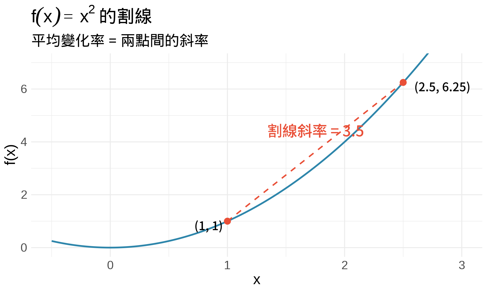
假設我們有一個函數 $f(x) = x^2$,想知道 $x=1$ 附近的變化率。
**平均變化率**定義為:
$$
\frac{f(x_1) - f(x_0)}{x_1 - x_0} = \frac{\Delta f}{\Delta x}
$$
這就是連接兩點的**割線斜率**。
```{r}
#| label: fig-secant-line
#| fig-cap: "割線斜率 = 平均變化率"
#| warning: false
#| message: false
f <- function(x) x^2
x0 <- 1
x1 <- 2.5
y0 <- f(x0)
y1 <- f(x1)

slope_secant <- (y1 - y0) / (x1 - x0)

x_range <- seq(-0.5, 3, by = 0.01)

ggplot() +
  # 原函數曲線
  geom_line(aes(x = x_range, y = f(x_range)),
            color = "#2E86AB", linewidth = 1.2) +
  # 割線
  geom_segment(aes(x = x0, y = y0, xend = x1, yend = y1),
               color = "#E94F37", linewidth = 1, linetype = "dashed") +
  # 兩個點
  geom_point(aes(x = c(x0, x1), y = c(y0, y1)),
             color = "#E94F37", size = 4) +
  # 標註
  annotate("text", x = 1.75, y = 4,
           label = paste0("割線斜率 = ", round(slope_secant, 2)),
           hjust = 0.5, vjust = -0.5, size = 5, color = "#E94F37") +
  annotate("text", x = x0, y = y0,
           label = paste0("(", x0, ", ", y0, ")"),
           hjust = 1.2, vjust = 1, size = 4) +
  annotate("text", x = x1, y = y1,
           label = paste0("(", x1, ", ", y1, ")"),
           hjust = -0.2, vjust = 1, size = 4) +
  labs(
    title = expression(f(x) == x^2 ~ "的割線"),
    subtitle = "平均變化率 = 兩點間的斜率",
    x = "x", y = "f(x)"
  ) +
  coord_cartesian(xlim = c(-0.5, 3), ylim = c(0, 7)) +
  theme_minimal(base_size = 14)
```
在這個例子中,從 $x=1$ 到 $x=2.5$,平均變化率是 $\frac{6.25-1}{2.5-1} = 3.5$。
但這只是**平均**,不能代表 $x=1$ 這一點的瞬時變化率。
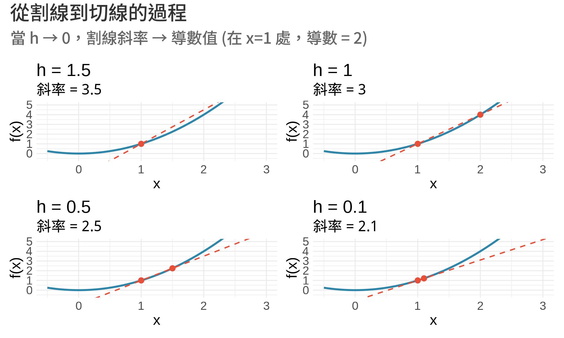
### 讓兩點越來越近:趨近切線
如果我們讓第二個點 $x_1$ 越來越接近 $x_0$,會發生什麼事?
```{r}
#| label: fig-secant-to-tangent
#| fig-cap: "當 h → 0,割線逐漸變成切線"
#| warning: false
#| message: false
f <- function(x) x^2
f_prime <- function(x) 2*x

x0 <- 1
y0 <- f(x0)

# 不同的 h 值
h_values <- c(1.5, 1, 0.5, 0.1)

plots <- lapply(h_values, function(h) {
  x1 <- x0 + h
  y1 <- f(x1)
  slope_secant <- (y1 - y0) / h

  x_range <- seq(-0.5, 3, by = 0.01)

  # 計算割線的延伸
  secant_intercept <- y0 - slope_secant * x0

  ggplot() +
    # 原函數
    geom_line(aes(x = x_range, y = f(x_range)),
              color = "#2E86AB", linewidth = 1.2) +
    # 割線(延伸到整個範圍)
    geom_abline(intercept = secant_intercept,
                slope = slope_secant,
                color = "#E94F37", linewidth = 0.8, linetype = "dashed") +
    # 兩點
    geom_point(aes(x = c(x0, x1), y = c(y0, y1)),
               color = "#E94F37", size = 3) +
    coord_cartesian(xlim = c(-0.5, 3), ylim = c(-0.5, 5)) +
    labs(
      title = paste0("h = ", h),
      subtitle = paste0("斜率 = ", round(slope_secant, 2)),
      x = "x", y = "f(x)"
    ) +
    theme_minimal(base_size = 12)
})

wrap_plots(plots, ncol = 2) +
  plot_annotation(
    title = "從割線到切線的過程",
    subtitle = "當 h → 0,割線斜率 → 導數值 (在 x=1 處,導數 = 2)",
    theme = theme(plot.title = element_text(size = 16, face = "bold"))
  )
```
觀察這四張圖,你會發現:
- 當 $h = 1.5$ 時,割線斜率 = 3.5
- 當 $h = 1$ 時,割線斜率 = 3
- 當 $h = 0.5$ 時,割線斜率 = 2.5
- 當 $h = 0.1$ 時,割線斜率 = 2.1
**斜率越來越接近 2**,這就是 $x=1$ 處的**切線斜率**,也就是**導數值**。
## 導數的數學定義
**導數 (derivative)** 定義為極限:
$$
f'(x) = \lim_{h \to 0} \frac{f(x+h) - f(x)}{h}
$$
這個定義可以用三種等價的形式表達:
| 符號 | 念法 | 使用時機 |
|------|------|----------|
| $f'(x)$ | "f prime of x" | 強調函數本身 |
| $\frac{df}{dx}$ | "df dx" | 強調變化率 |
| $\frac{dy}{dx}$ | "dy dx" | 當 $y = f(x)$ 時 |
:::{.callout-note}
## 為什麼用 $h$ 而不是 $\Delta x$?
傳統上,$\Delta x$ 表示「有限的變化量」,而 $h$ 強調「趨近於 0 的微小量」。兩者概念相同,只是習慣不同。
:::
### 範例:計算 $f(x) = x^2$ 在 $x=1$ 的導數
使用定義:
$$
\begin{align}
f'(1) &= \lim_{h \to 0} \frac{f(1+h) - f(1)}{h} \\
&= \lim_{h \to 0} \frac{(1+h)^2 - 1^2}{h} \\
&= \lim_{h \to 0} \frac{1 + 2h + h^2 - 1}{h} \\
&= \lim_{h \to 0} \frac{2h + h^2}{h} \\
&= \lim_{h \to 0} (2 + h) \\
&= 2
\end{align}
$$
這驗證了我們視覺化看到的結果!
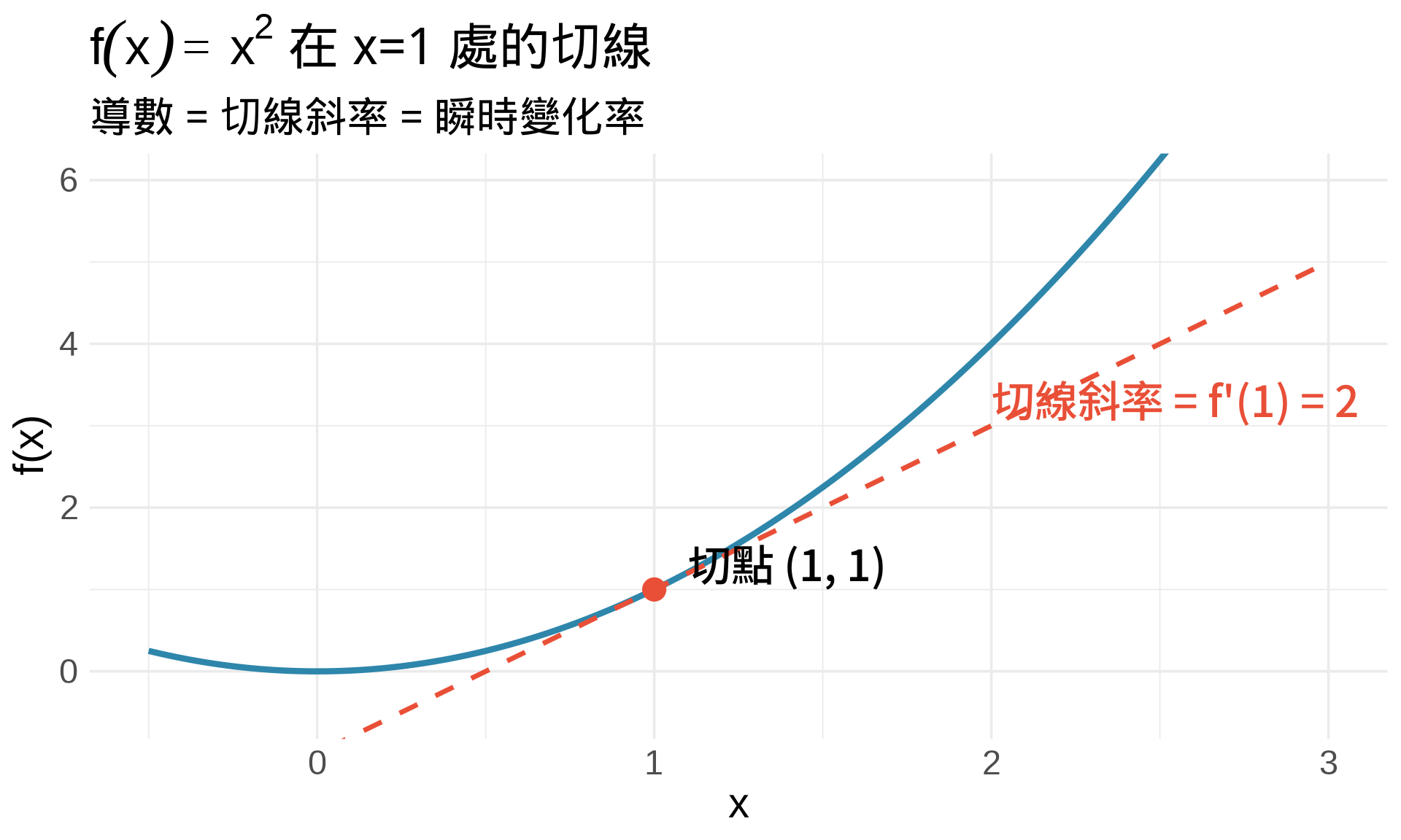
## 導數的幾何意義
導數有兩種等價的幾何解釋:
1. **切線斜率**:$f'(x)$ 是曲線在 $(x, f(x))$ 處的切線斜率
2. **瞬時變化率**:$f'(x)$ 是 $y$ 對 $x$ 的瞬時變化速度
```{r}
#| label: fig-tangent-interpretation
#| fig-cap: "導數的幾何意義:切線斜率"
#| warning: false
#| message: false
f <- function(x) x^2
f_prime <- function(x) 2*x

x0 <- 1
y0 <- f(x0)
slope <- f_prime(x0)

# 切線方程式:y - y0 = slope * (x - x0)
tangent <- function(x) y0 + slope * (x - x0)

x_range <- seq(-0.5, 3, by = 0.01)

ggplot() +
  # 原函數
  geom_line(aes(x = x_range, y = f(x_range)),
            color = "#2E86AB", linewidth = 1.5) +
  # 切線
  geom_line(aes(x = x_range, y = tangent(x_range)),
            color = "#E94F37", linewidth = 1.2, linetype = "dashed") +
  # 切點
  geom_point(aes(x = x0, y = y0),
             color = "#E94F37", size = 5) +
  # 標註
  annotate("text", x = x0 + 0.1, y = y0 + 0.3,
           label = paste0("切點 (", x0, ", ", y0, ")"),
           hjust = 0, size = 5) +
  annotate("text", x = 2, y = tangent(2) + 0.3,
           label = paste0("切線斜率 = f'(1) = ", slope),
           hjust = 0, size = 5, color = "#E94F37") +
  labs(
    title = expression(f(x) == x^2 ~ "在 x=1 處的切線"),
    subtitle = "導數 = 切線斜率 = 瞬時變化率",
    x = "x", y = "f(x)"
  ) +
  coord_cartesian(xlim = c(-0.5, 3), ylim = c(-0.5, 6)) +
  theme_minimal(base_size = 14)
```
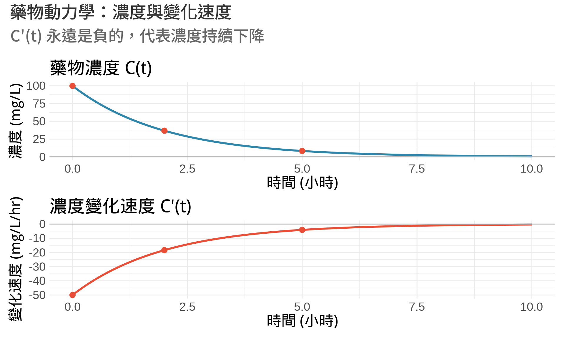
## 導數的物理意義:藥物動力學範例
假設某藥物在體內的濃度隨時間變化為:
$$
C(t) = 100 \cdot e^{-0.5t} \quad \text{(單位:mg/L)}
$$
導數 $C'(t)$ 代表**濃度的變化速度**(單位:mg/L/hr)。
```{r}
#| label: fig-drug-kinetics
#| fig-cap: "藥物濃度與其變化速度"
#| warning: false
#| message: false
# 藥物濃度函數
C <- function(t) 100 * exp(-0.5 * t)
C_prime <- function(t) -50 * exp(-0.5 * t)

t <- seq(0, 10, by = 0.1)

df <- data.frame(
  t = t,
  C = C(t),
  C_prime = C_prime(t)
)

p1 <- ggplot(df, aes(t, C)) +
  geom_line(color = "#2E86AB", linewidth = 1.2) +
  geom_hline(yintercept = 0, color = "gray70") +
  # 標記幾個時間點
  geom_point(data = data.frame(t = c(0, 2, 5), C = C(c(0, 2, 5))),
             aes(t, C), color = "#E94F37", size = 3) +
  labs(
    title = "藥物濃度 C(t)",
    x = "時間 (小時)", y = "濃度 (mg/L)"
  ) +
  theme_minimal(base_size = 12)

p2 <- ggplot(df, aes(t, C_prime)) +
  geom_line(color = "#E94F37", linewidth = 1.2) +
  geom_hline(yintercept = 0, color = "gray70") +
  geom_point(data = data.frame(t = c(0, 2, 5), C_prime = C_prime(c(0, 2, 5))),
             aes(t, C_prime), color = "#E94F37", size = 3) +
  labs(
    title = "濃度變化速度 C'(t)",
    x = "時間 (小時)", y = "變化速度 (mg/L/hr)"
  ) +
  theme_minimal(base_size = 12)

p1 / p2 +
  plot_annotation(
    title = "藥物動力學:濃度與變化速度",
    subtitle = "C'(t) 永遠是負的,代表濃度持續下降",
    theme = theme(plot.title = element_text(size = 14, face = "bold"))
  )
```
**解讀**:
- 在 $t=0$ 時,$C'(0) = -50$ mg/L/hr,代表濃度正以每小時 50 mg/L 的速度下降
- 隨著時間增加,$|C'(t)|$ 越來越小,代表下降速度越來越慢
- 這符合藥物代謝的一般規律:濃度越高,代謝越快
## 統計應用
### 1. Hazard Rate(風險函數)
在存活分析中,**hazard function** $h(t)$ 定義為:
$$
h(t) = \lim_{\Delta t \to 0} \frac{P(t \le T < t + \Delta t \mid T \ge t)}{\Delta t}
$$
這就是**瞬時死亡率**,是導數概念的直接應用!
事實上,hazard function 可以用機率密度函數 $f(t)$ 和存活函數 $S(t)$ 表示:
$$
h(t) = \frac{f(t)}{S(t)} = -\frac{d}{dt} \ln S(t)
$$
### 2. Score Function(計分函數)
在最大概似估計中,**score function** 定義為 log-likelihood 對參數的導數:
$$
U(\theta) = \frac{d}{d\theta} \ell(\theta)
$$
MLE 的核心想法就是:**令 score function = 0**,找到讓 likelihood 最大的 $\theta$。
### 3. Gradient Descent(梯度下降法)
機器學習中的優化演算法,利用導數決定參數更新方向:
$$
\theta_{new} = \theta_{old} - \alpha \cdot \frac{d}{d\theta} L(\theta)
$$
其中 $\alpha$ 是學習率,$\frac{d}{d\theta} L(\theta)$ 是損失函數的導數(梯度)。
## 練習題
### 觀念題
1. 用自己的話解釋:「導數」和「平均變化率」有什麼不同?
::: {.callout-tip collapse="true" title="參考答案"}
平均變化率是兩點之間的變化量(割線斜率),而導數是某一點的瞬時變化率(切線斜率)。平均變化率描述一段區間的整體趨勢,導數則精確描述某一時刻的變化速度。就像計算平均速度 vs 瞬時速度的差別。
:::
2. 為什麼存活分析需要「瞬時」死亡率,而不是「平均」死亡率?
::: {.callout-tip collapse="true" title="參考答案"}
因為死亡風險會隨時間變化,平均死亡率無法捕捉特定時刻的風險高低。例如,手術後第一週的風險可能很高,但第一年的平均風險卻可能看起來不高。hazard rate 提供了每個時刻的精確風險,這對臨床決策非常重要。
:::
3. 如果 $f'(x) > 0$,代表函數在該點是上升還是下降?
::: {.callout-tip collapse="true" title="參考答案"}
上升。導數代表切線斜率,$f'(x) > 0$ 表示斜率為正,函數在該點呈現上升趨勢。反之,$f'(x) < 0$ 代表下降,$f'(x) = 0$ 代表水平(可能是極值點)。
:::
### 計算題
4. 使用導數的定義,計算 $f(x) = 3x$ 在 $x=2$ 的導數。
::: {.callout-tip collapse="true" title="參考答案"}
使用定義:$f'(2) = \lim_{h \to 0} \frac{f(2+h) - f(2)}{h} = \lim_{h \to 0} \frac{3(2+h) - 3(2)}{h} = \lim_{h \to 0} \frac{6+3h-6}{h} = \lim_{h \to 0} 3 = 3$。線性函數的導數就是斜率,所以 $f'(x) = 3$ 在所有點都成立。
:::
5. 如果藥物濃度 $C(t) = 50e^{-0.3t}$,計算 $t=1$ 時的變化速度。
::: {.callout-tip collapse="true" title="參考答案"}
導數為 $C'(t) = 50 \times (-0.3) \times e^{-0.3t} = -15e^{-0.3t}$。在 $t=1$ 時,$C'(1) = -15e^{-0.3} \approx -11.1$ mg/L/hr。負號代表濃度正在下降,在第 1 小時時以每小時約 11.1 mg/L 的速度減少。
:::
### R 操作題
6. 修改藥物動力學範例的程式碼,改成 $C(t) = 80e^{-0.4t}$,觀察變化速度圖的差異。
::: {.callout-tip collapse="true" title="參考答案"}
將程式碼改為 `C <- function(t) 80 * exp(-0.4 * t)` 和 `C_prime <- function(t) -32 * exp(-0.4 * t)`。你會觀察到:初始濃度較高(80 vs 100)、下降速度較快(係數 -0.4 vs -0.5),且變化速度圖的起始值為 -32(更陡峭的下降)。
:::
```{r}
#| eval: false
# 你的程式碼
C <- function(t) ___
C_prime <- function(t) ___
```
7. 繪製 $f(x) = x^3$ 在 $x=1$ 處的割線(使用 $h=0.5$)和切線,比較差異。
::: {.callout-tip collapse="true" title="參考答案"}
對於 $f(x) = x^3$,在 $x=1$ 的導數為 $f'(1) = 3$(切線斜率)。而割線連接 $(1, 1)$ 和 $(1.5, 3.375)$,斜率為 $(3.375-1)/0.5 = 4.75$。你會看到割線比切線更陡,因為它高估了瞬時變化率。隨著 $h$ 減小,割線會越來越接近切線。
:::
## 本章重點整理 {.unnumbered}
:::{.callout-important}
## Key Takeaways
1. **導數 = 瞬時變化率 = 切線斜率**:三種理解方式本質相同
2. **從割線到切線**:讓兩點距離趨近於零,割線斜率趨近切線斜率
3. **導數定義**:$f'(x) = \lim_{h \to 0} \frac{f(x+h) - f(x)}{h}$
4. **醫學統計應用**:
- Hazard rate 是瞬時死亡率(導數概念)
- Score function 是 MLE 的核心工具(對參數微分)
- Gradient descent 利用導數優化參數(機器學習)
5. **下一章預告**:我們會學習快速計算導數的規則,不用每次都用定義!
:::