# 最佳化 (Optimization)
```{r}
#| include: false
source(here::here("R/_common.R"))
```
## 學習目標 {.unnumbered}
- 用導數找函數的極值點:令 $f'(x) = 0$
- 使用二階導數判斷極大或極小
- 理解凹向上 (concave up) 與凹向下 (concave down)
- 連結醫學統計:MLE、最小平方法、梯度下降法
## 為什麼需要最佳化?
統計學的核心問題之一就是**找最佳值**:
- **最大概似估計 (MLE)**:找讓 likelihood 最大的參數值
- **最小平方法 (OLS)**:找讓殘差平方和最小的迴歸係數
- **機器學習**:找讓損失函數最小的模型參數
這些都是**最佳化問題 (optimization problems)**,而微分是解決這類問題的關鍵工具!
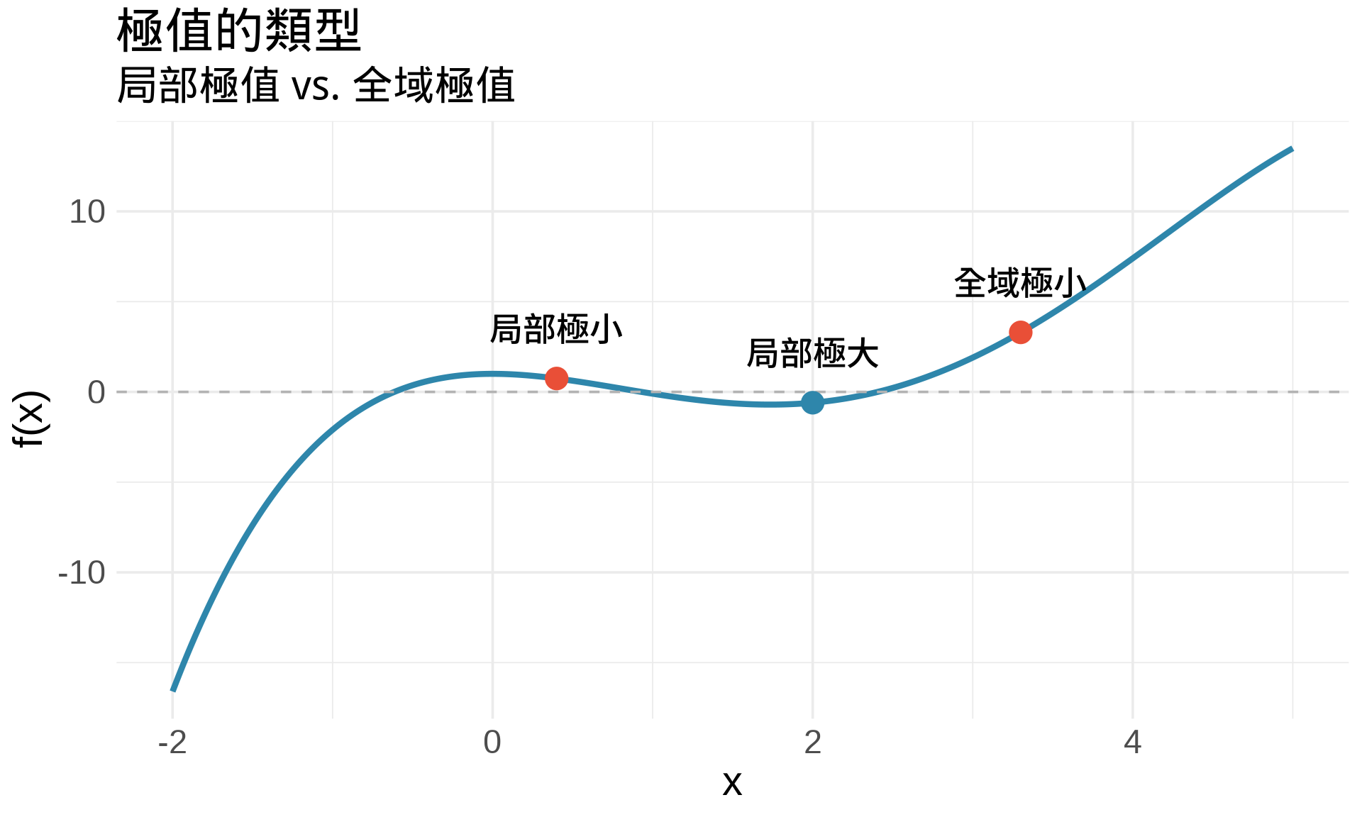
## 極值的基本概念
### 什麼是極值?
**局部極大值 (local maximum)**:在某個範圍內,函數值最大的點
**局部極小值 (local minimum)**:在某個範圍內,函數值最小的點
**全域極值 (global extrema)**:在整個定義域內的最大或最小值
```{r}
#| label: fig-extrema-concept
#| fig-cap: "極值的視覺化:局部與全域"
#| warning: false
#| message: false
# 創建一個有多個極值的函數
f <- function(x) {
  -0.1*x^4 + x^3 - 2*x^2 + 1
}

x <- seq(-2, 5, by = 0.01)
y <- f(x)

df <- data.frame(x, y)

# 找極值點(數值近似)
# 局部極小值約在 x ≈ 0.4 和 x ≈ 3.3
# 局部極大值約在 x ≈ 2
extrema <- data.frame(
  x = c(0.4, 2, 3.3),
  y = f(c(0.4, 2, 3.3)),
  type = c("局部極小", "局部極大", "全域極小"),
  color = c("#E94F37", "#2E86AB", "#E94F37")
)

ggplot(df, aes(x, y)) +
  geom_line(color = "#2E86AB", linewidth = 1.5) +
  geom_hline(yintercept = 0, color = "gray70", linetype = "dashed") +
  geom_point(data = extrema, aes(x, y, color = type), size = 5) +
  geom_text(data = extrema, aes(x, y, label = type),
            vjust = -1.5, size = 4, fontface = "bold") +
  scale_color_manual(values = c("局部極大" = "#2E86AB",
                                "局部極小" = "#E94F37",
                                "全域極小" = "#E94F37")) +
  labs(
    title = "極值的類型",
    subtitle = "局部極值 vs. 全域極值",
    x = "x", y = "f(x)"
  ) +
  theme_minimal(base_size = 14) +
  theme(legend.position = "none")
```
## 一階導數檢定 (First Derivative Test)
### 核心定理
**Fermat's Theorem**:如果 $f(x)$ 在 $x=c$ 有局部極值,且 $f'(c)$ 存在,則:
$$
f'(c) = 0
$$
**白話文**:極值點的切線斜率是水平的(斜率 = 0)。
:::{.callout-note}
## 注意
$f'(c) = 0$ 是極值的**必要條件**,但不是**充分條件**。
也就是說:
- 極值點 $\Rightarrow$ $f'(c) = 0$(一定成立)
- $f'(c) = 0$ $\nRightarrow$ 極值點(不一定成立)
反例:$f(x) = x^3$ 在 $x=0$ 處,$f'(0) = 0$,但這不是極值點!
:::
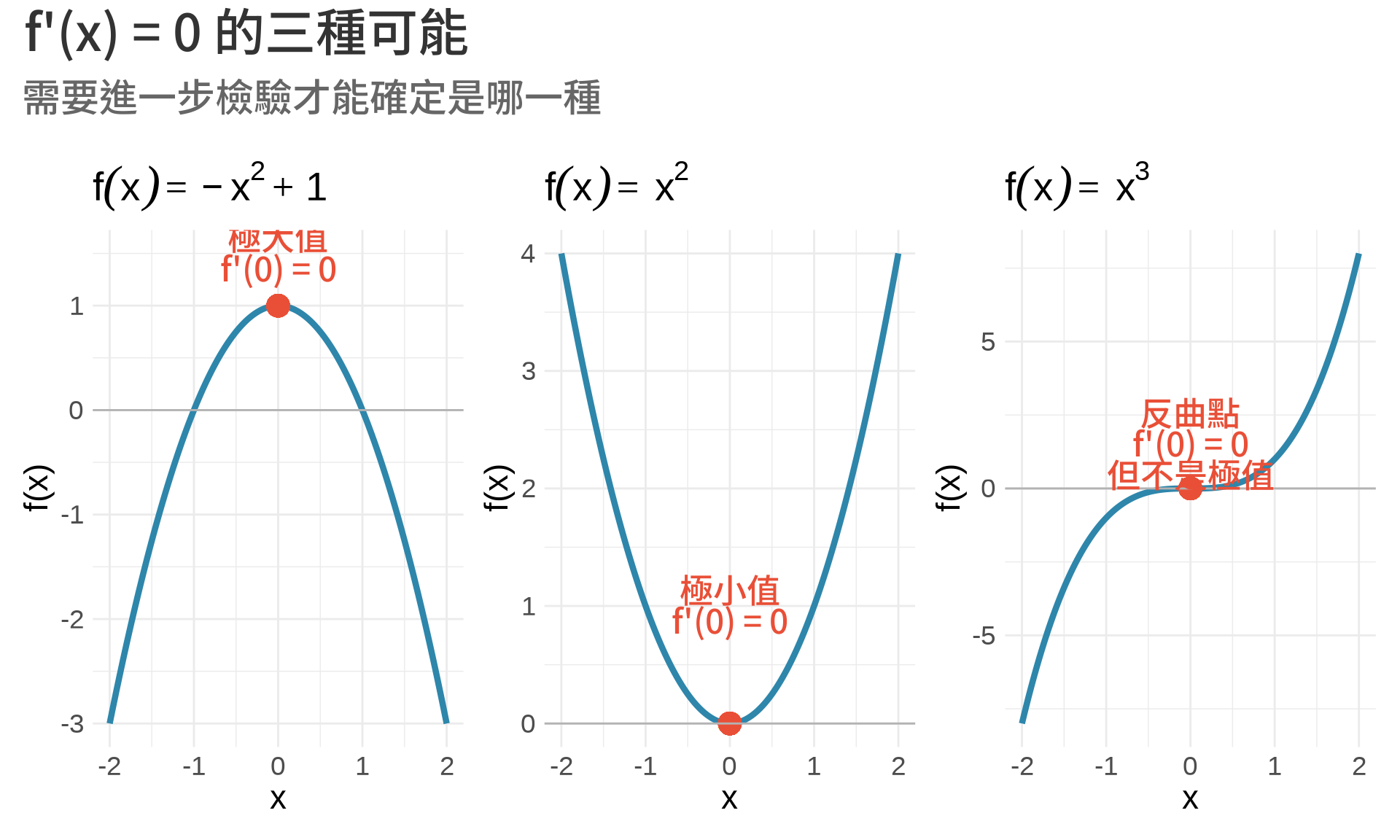
### 找極值點的步驟
1. 計算導數 $f'(x)$
2. 解方程式 $f'(x) = 0$,找出**臨界點 (critical points)**
3. 判斷每個臨界點是極大、極小、還是反曲點
```{r}
#| label: fig-critical-points
#| fig-cap: "臨界點的三種類型"
#| warning: false
#| message: false
x <- seq(-2, 2, by = 0.01)

# 三種情況
f1 <- -x^2 + 1       # 極大值
f2 <- x^2            # 極小值
f3 <- x^3            # 反曲點

df <- data.frame(x, f1, f2, f3)

p1 <- ggplot(df, aes(x, f1)) +
  geom_line(color = "#2E86AB", linewidth = 1.5) +
  geom_point(aes(x = 0, y = 1), color = "#E94F37", size = 5) +
  geom_hline(yintercept = 0, color = "gray70") +
  annotate("text", x = 0, y = 1.5, label = "極大值\nf'(0) = 0",
           hjust = 0.5, color = "#E94F37", fontface = "bold") +
  labs(title = expression(f(x) == -x^2 + 1), y = "f(x)") +
  theme_minimal(base_size = 11)

p2 <- ggplot(df, aes(x, f2)) +
  geom_line(color = "#2E86AB", linewidth = 1.5) +
  geom_point(aes(x = 0, y = 0), color = "#E94F37", size = 5) +
  geom_hline(yintercept = 0, color = "gray70") +
  annotate("text", x = 0, y = 1, label = "極小值\nf'(0) = 0",
           hjust = 0.5, color = "#E94F37", fontface = "bold") +
  labs(title = expression(f(x) == x^2), y = "f(x)") +
  theme_minimal(base_size = 11)

p3 <- ggplot(df, aes(x, f3)) +
  geom_line(color = "#2E86AB", linewidth = 1.5) +
  geom_point(aes(x = 0, y = 0), color = "#E94F37", size = 5) +
  geom_hline(yintercept = 0, color = "gray70") +
  annotate("text", x = 0, y = 1.5, label = "反曲點\nf'(0) = 0\n但不是極值",
           hjust = 0.5, color = "#E94F37", fontface = "bold") +
  labs(title = expression(f(x) == x^3), y = "f(x)") +
  theme_minimal(base_size = 11)

(p1 | p2 | p3) +
  plot_annotation(
    title = "f'(x) = 0 的三種可能",
    subtitle = "需要進一步檢驗才能確定是哪一種"
  )
```
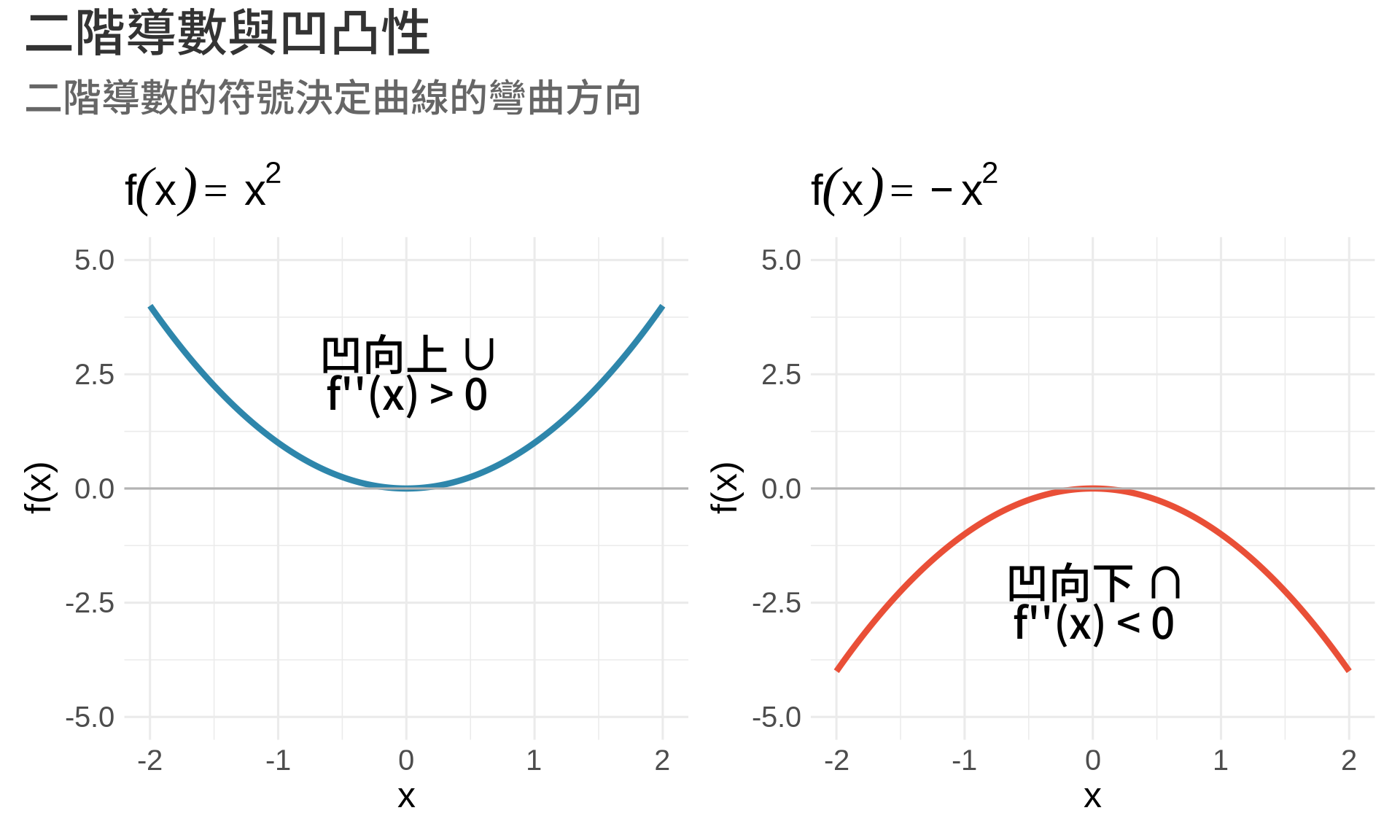
## 二階導數檢定 (Second Derivative Test)
### 凹向上與凹向下
**二階導數** $f''(x)$ 描述函數的**彎曲方向**:
- $f''(x) > 0$:函數**凹向上 (concave up)**,像微笑 ∪
- $f''(x) < 0$:函數**凹向下 (concave down)**,像皺眉 ∩
```{r}
#| label: fig-concavity
#| fig-cap: "凹向上 vs. 凹向下"
#| warning: false
#| message: false
x <- seq(-2, 2, by = 0.01)

f_up <- x^2           # f''(x) = 2 > 0
f_down <- -x^2        # f''(x) = -2 < 0

df <- data.frame(x, f_up, f_down)

p1 <- ggplot(df, aes(x, f_up)) +
  geom_line(color = "#2E86AB", linewidth = 1.5) +
  geom_hline(yintercept = 0, color = "gray70") +
  annotate("text", x = 0, y = 2.5, label = "凹向上 ∪\nf''(x) > 0",
           hjust = 0.5, size = 5, fontface = "bold") +
  labs(title = expression(f(x) == x^2), y = "f(x)") +
  ylim(-5, 5) +
  theme_minimal(base_size = 12)

p2 <- ggplot(df, aes(x, f_down)) +
  geom_line(color = "#E94F37", linewidth = 1.5) +
  geom_hline(yintercept = 0, color = "gray70") +
  annotate("text", x = 0, y = -2.5, label = "凹向下 ∩\nf''(x) < 0",
           hjust = 0.5, size = 5, fontface = "bold") +
  labs(title = expression(f(x) == -x^2), y = "f(x)") +
  ylim(-5, 5) +
  theme_minimal(base_size = 12)

p1 + p2 +
  plot_annotation(
    title = "二階導數與凹凸性",
    subtitle = "二階導數的符號決定曲線的彎曲方向"
  )
```
### 二階導數檢定
假設 $f'(c) = 0$(臨界點),則:
| $f''(c)$ | 結論 |
|----------|------|
| $f''(c) > 0$ | $c$ 是**局部極小值** |
| $f''(c) < 0$ | $c$ 是**局部極大值** |
| $f''(c) = 0$ | **無法判斷**,需要其他方法 |
**直觀理解**:
- 凹向上 ($f'' > 0$) + 水平切線 ($f' = 0$) = 谷底(極小值)
- 凹向下 ($f'' < 0$) + 水平切線 ($f' = 0$) = 山頂(極大值)
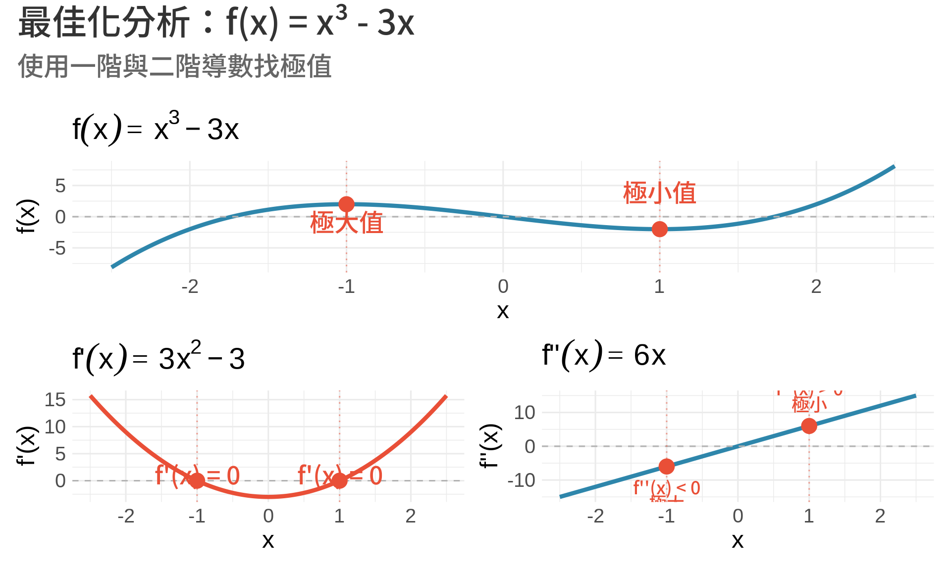
### 範例:找 $f(x) = x^3 - 3x$ 的極值
**步驟 1**:計算一階導數
$$
f'(x) = 3x^2 - 3
$$
**步驟 2**:找臨界點
$$
f'(x) = 0 \Rightarrow 3x^2 - 3 = 0 \Rightarrow x^2 = 1 \Rightarrow x = \pm 1
$$
**步驟 3**:計算二階導數
$$
f''(x) = 6x
$$
**步驟 4**:判斷極值類型
- 在 $x = -1$:$f''(-1) = -6 < 0$ → **極大值**,$f(-1) = 2$
- 在 $x = 1$:$f''(1) = 6 > 0$ → **極小值**,$f(1) = -2$
```{r}
#| label: fig-optimization-example
#| fig-cap: "完整的最佳化分析"
#| warning: false
#| message: false
x <- seq(-2.5, 2.5, by = 0.01)

f <- x^3 - 3*x
f_prime <- 3*x^2 - 3
f_double_prime <- 6*x

df <- data.frame(x, f, f_prime, f_double_prime)

# 極值點
extrema <- data.frame(
  x = c(-1, 1),
  y = c(2, -2),
  type = c("極大值", "極小值")
)

p1 <- ggplot(df, aes(x, f)) +
  geom_line(color = "#2E86AB", linewidth = 1.5) +
  geom_hline(yintercept = 0, color = "gray70", linetype = "dashed") +
  geom_vline(xintercept = c(-1, 1), color = "#E94F37",
             linetype = "dotted", alpha = 0.5) +
  geom_point(data = extrema, aes(x, y), color = "#E94F37", size = 5) +
  geom_text(data = extrema, aes(x, y, label = type),
            vjust = c(1.5, -1.5), hjust = 0.5, color = "#E94F37",
            fontface = "bold") +
  labs(title = expression(f(x) == x^3 - 3*x), y = "f(x)") +
  theme_minimal(base_size = 12)

zeros_df <- data.frame(x = c(-1, 1), y = c(0, 0))

p2 <- ggplot(df, aes(x, f_prime)) +
  geom_line(color = "#E94F37", linewidth = 1.5) +
  geom_hline(yintercept = 0, color = "gray70", linetype = "dashed") +
  geom_vline(xintercept = c(-1, 1), color = "#E94F37",
             linetype = "dotted", alpha = 0.5) +
  geom_point(data = zeros_df, aes(x = x, y = y),
             color = "#E94F37", size = 5) +
  annotate("text", x = c(-1, 1), y = c(1, 1),
           label = "f'(x) = 0", hjust = 0.5, color = "#E94F37") +
  labs(title = expression(f*"'"*(x) == 3*x^2 - 3), y = "f'(x)") +
  theme_minimal(base_size = 12)

second_df <- data.frame(x = c(-1, 1), y = c(-6, 6))

p3 <- ggplot(df, aes(x, f_double_prime)) +
  geom_line(color = "#2E86AB", linewidth = 1.5) +
  geom_hline(yintercept = 0, color = "gray70", linetype = "dashed") +
  geom_vline(xintercept = c(-1, 1), color = "#E94F37",
             linetype = "dotted", alpha = 0.5) +
  geom_point(data = second_df, aes(x = x, y = y),
             color = "#E94F37", size = 5) +
  annotate("text", x = -1, y = -6, label = "f''(x) < 0\n極大",
           vjust = 1.5, hjust = 0.5, color = "#E94F37", size = 3) +
  annotate("text", x = 1, y = 6, label = "f''(x) > 0\n極小",
           vjust = -0.5, hjust = 0.5, color = "#E94F37", size = 3) +
  labs(title = expression(f*"''"*(x) == 6*x), y = "f''(x)") +
  theme_minimal(base_size = 12)

p1 / (p2 + p3) +
  plot_annotation(
    title = "最佳化分析:f(x) = x³ - 3x",
    subtitle = "使用一階與二階導數找極值"
  )
```
## 統計應用
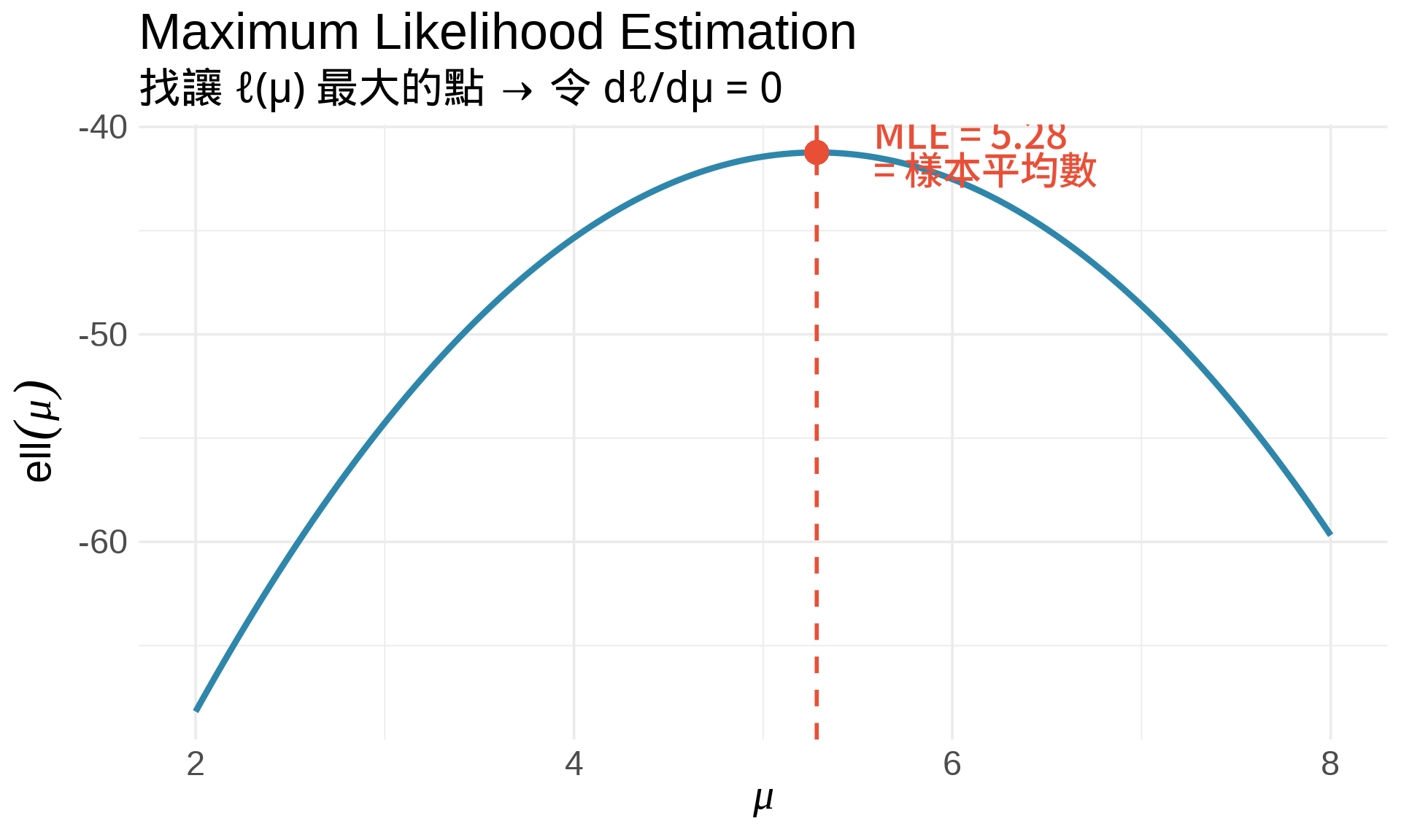
### 1. 最大概似估計 (MLE)
**核心想法**:找讓 likelihood 最大的參數值。
**步驟**:
1. 寫出 likelihood function:$L(\theta) = \prod_{i=1}^n f(x_i; \theta)$
2. 取對數:$\ell(\theta) = \ln L(\theta) = \sum_{i=1}^n \ln f(x_i; \theta)$
3. 對 $\theta$ 微分:$\frac{d\ell}{d\theta}$
4. 令導數為 0:$\frac{d\ell}{d\theta} = 0$
5. 解出 $\hat{\theta}_{\text{MLE}}$
**範例:估計常態分布的平均數**
假設 $X_1, \ldots, X_n \sim N(\mu, \sigma^2)$,已知 $\sigma^2$,要估計 $\mu$。
$$
\begin{align}
\ell(\mu) &= \sum_{i=1}^n \ln f(x_i; \mu) \\
&= \sum_{i=1}^n \ln \left[\frac{1}{\sqrt{2\pi\sigma^2}} \exp\left(-\frac{(x_i - \mu)^2}{2\sigma^2}\right)\right] \\
&= -\frac{n}{2}\ln(2\pi\sigma^2) - \frac{1}{2\sigma^2}\sum_{i=1}^n (x_i - \mu)^2
\end{align}
$$
**微分**:
$$
\frac{d\ell}{d\mu} = \frac{1}{\sigma^2}\sum_{i=1}^n (x_i - \mu)
$$
**令導數為 0**:
$$
\sum_{i=1}^n (x_i - \mu) = 0 \Rightarrow \hat{\mu}_{\text{MLE}} = \frac{1}{n}\sum_{i=1}^n x_i = \bar{x}
$$
**結論**:樣本平均數就是 MLE!
```{r}
#| label: fig-mle-normal
#| fig-cap: "MLE 視覺化:找讓 log-likelihood 最大的 μ"
#| warning: false
#| message: false
set.seed(123)
data <- rnorm(20, mean = 5, sd = 2)

# Log-likelihood 函數(固定 sigma = 2)
log_lik <- function(mu) {
  sum(dnorm(data, mean = mu, sd = 2, log = TRUE))
}

mu_range <- seq(2, 8, by = 0.01)
ll_values <- sapply(mu_range, log_lik)

# MLE
mu_mle <- mean(data)
ll_mle <- log_lik(mu_mle)

df <- data.frame(mu = mu_range, ll = ll_values)

ggplot(df, aes(mu, ll)) +
  geom_line(color = "#2E86AB", linewidth = 1.5) +
  geom_vline(xintercept = mu_mle, color = "#E94F37",
             linetype = "dashed", linewidth = 1) +
  geom_point(aes(x = mu_mle, y = ll_mle),
             color = "#E94F37", size = 5) +
  annotate("text", x = mu_mle + 0.3, y = ll_mle,
           label = paste0("MLE = ", round(mu_mle, 2), "\n= 樣本平均數"),
           hjust = 0, vjust = 0.5, color = "#E94F37",
           fontface = "bold", size = 4.5) +
  labs(
    title = "Maximum Likelihood Estimation",
    subtitle = "找讓 ℓ(μ) 最大的點 → 令 dℓ/dμ = 0",
    x = expression(mu),
    y = expression(ell(mu))
  ) +
  theme_minimal(base_size = 14)
```
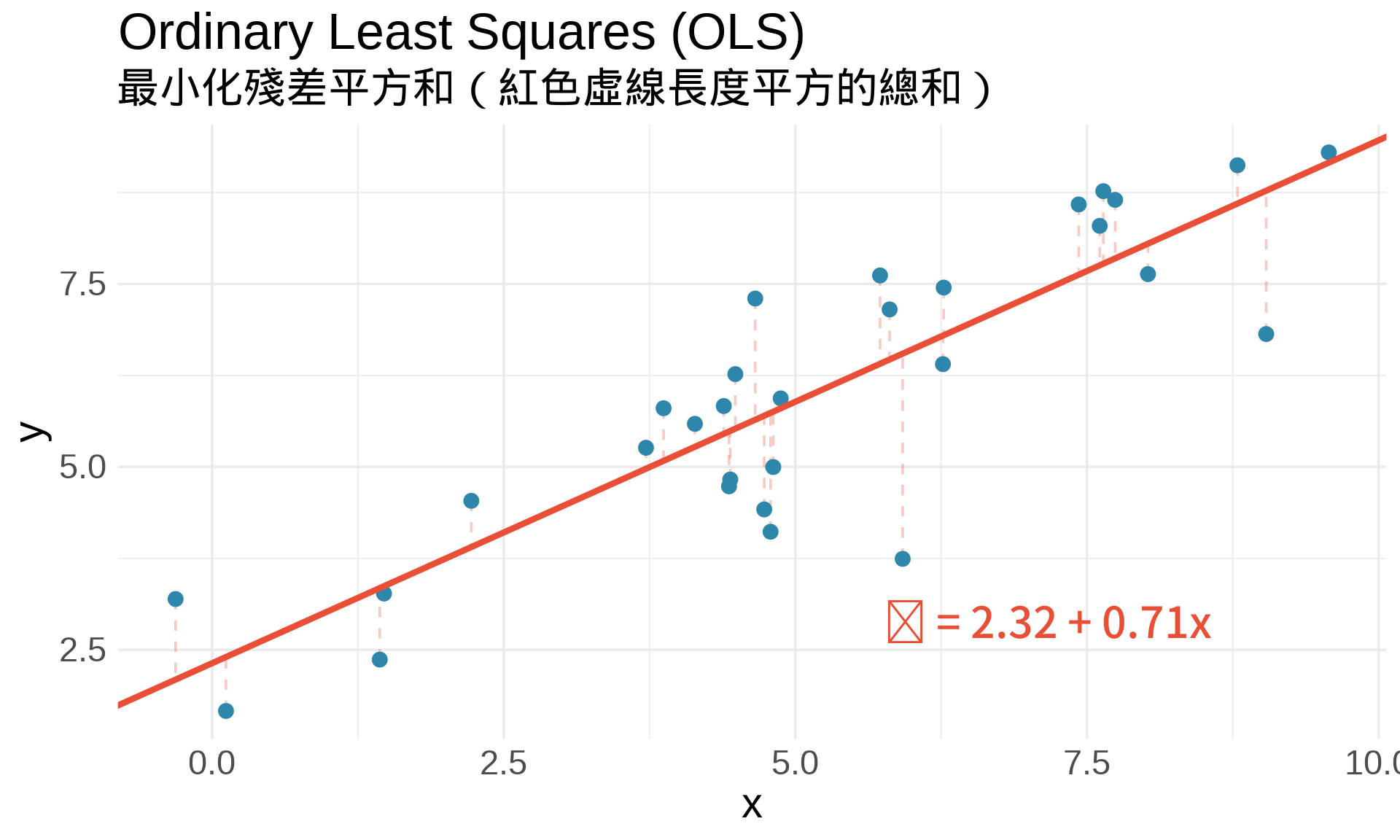
### 2. 最小平方法 (Ordinary Least Squares)
在簡單線性迴歸中:
$$
y_i = \beta_0 + \beta_1 x_i + \epsilon_i
$$
**目標**:找 $\beta_0, \beta_1$ 使**殘差平方和 (RSS)** 最小:
$$
\text{RSS}(\beta_0, \beta_1) = \sum_{i=1}^n (y_i - \beta_0 - \beta_1 x_i)^2
$$
**最佳化條件**:
$$
\frac{\partial \text{RSS}}{\partial \beta_0} = 0, \quad \frac{\partial \text{RSS}}{\partial \beta_1} = 0
$$
解出來就是**最小平方估計式**!
```{r}
#| label: fig-ols-visualization
#| fig-cap: "OLS:找讓 RSS 最小的迴歸線"
#| warning: false
#| message: false
set.seed(42)
n <- 30
x <- rnorm(n, mean = 5, sd = 2)
y <- 2 + 0.8*x + rnorm(n, sd = 1)

# 計算 OLS
fit <- lm(y ~ x)
beta0_hat <- coef(fit)[1]
beta1_hat <- coef(fit)[2]

df <- data.frame(x, y, y_pred = predict(fit))

ggplot(df, aes(x, y)) +
  geom_segment(aes(xend = x, yend = y_pred),
               color = "#E94F37", alpha = 0.3, linetype = "dashed") +
  geom_point(color = "#2E86AB", size = 3) +
  geom_abline(intercept = beta0_hat, slope = beta1_hat,
              color = "#E94F37", linewidth = 1.5) +
  annotate("text", x = max(x) - 1, y = min(y) + 1,
           label = paste0("ŷ = ", round(beta0_hat, 2), " + ",
                         round(beta1_hat, 2), "x"),
           hjust = 1, vjust = 0, color = "#E94F37",
           fontface = "bold", size = 5) +
  labs(
    title = "Ordinary Least Squares (OLS)",
    subtitle = "最小化殘差平方和(紅色虛線長度平方的總和)",
    x = "x", y = "y"
  ) +
  theme_minimal(base_size = 14)
```
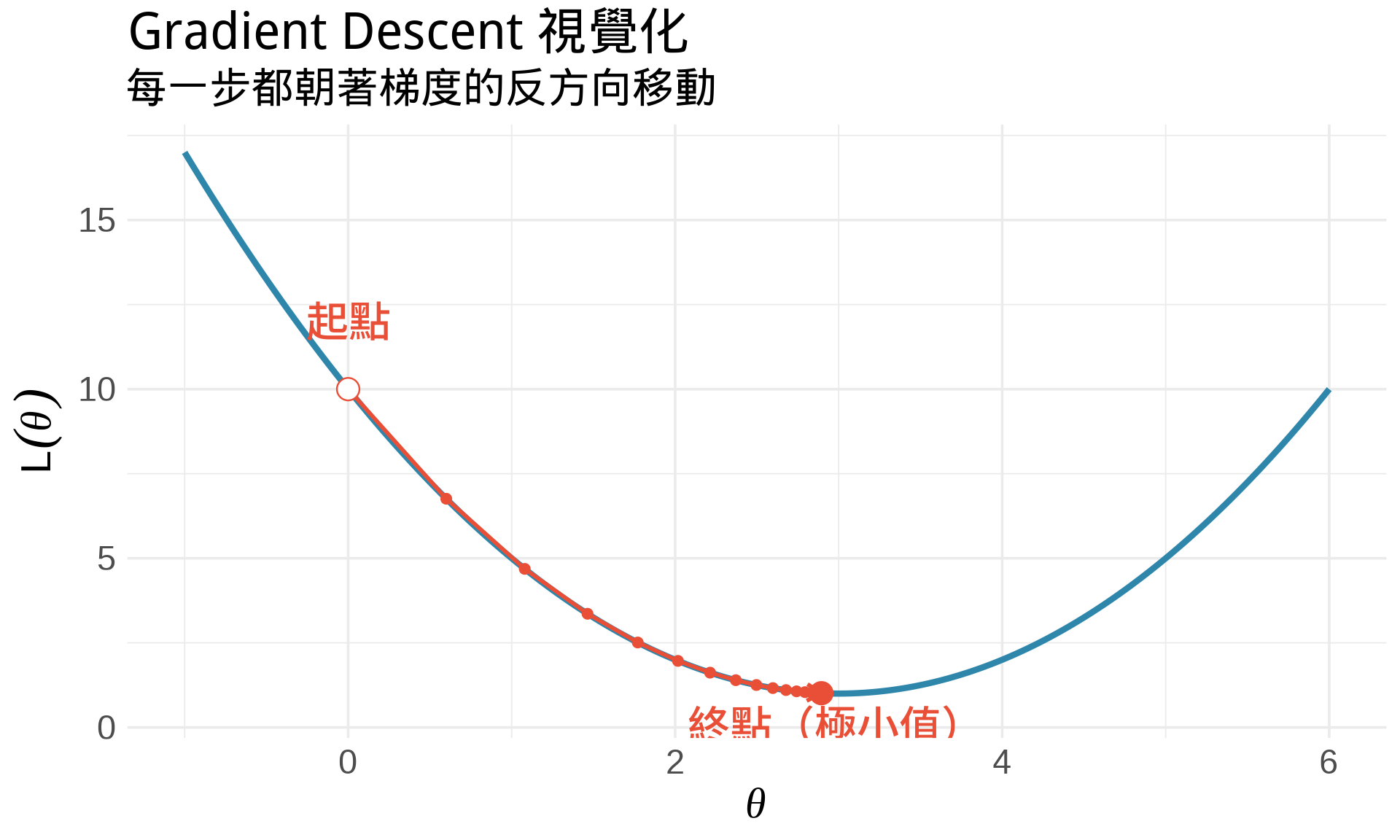
### 3. 梯度下降法 (Gradient Descent)
在機器學習中,有些損失函數無法直接解析求解,需要用**迭代法**。
**梯度下降法**的核心想法:
1. 從某個初始值 $\theta_0$ 開始
2. 計算梯度(導數):$g = \frac{d}{d\theta}L(\theta)$
3. 朝著梯度的**反方向**移動:$\theta_{t+1} = \theta_t - \alpha \cdot g_t$
4. 重複直到收斂
其中 $\alpha$ 叫做**學習率 (learning rate)**。
**直觀理解**:想像你在山上,想找到最低點。你看不到全貌,只能感受腳下的斜率。你每次都往下坡走一小步,最終會到達谷底。
```{r}
#| label: fig-gradient-descent
#| fig-cap: "梯度下降法的視覺化"
#| warning: false
#| message: false
# 簡單的二次函數
f <- function(x) (x - 3)^2 + 1
f_prime <- function(x) 2*(x - 3)

# 梯度下降
gradient_descent <- function(x0, alpha, n_iter) {
  path <- numeric(n_iter + 1)
  path[1] <- x0

  for (i in 1:n_iter) {
    grad <- f_prime(path[i])
    path[i+1] <- path[i] - alpha * grad
  }

  data.frame(
    iter = 0:n_iter,
    x = path,
    y = f(path)
  )
}

# 執行梯度下降
path <- gradient_descent(x0 = 0, alpha = 0.1, n_iter = 15)

x <- seq(-1, 6, by = 0.01)

ggplot() +
  # 函數曲線
  geom_line(aes(x = x, y = f(x)), color = "#2E86AB", linewidth = 1.5) +
  # 梯度下降路徑
  geom_path(data = path, aes(x, y), color = "#E94F37",
            linewidth = 1, arrow = arrow(length = unit(0.3, "cm"))) +
  geom_point(data = path, aes(x, y), color = "#E94F37", size = 2) +
  # 起點和終點
  geom_point(data = path[1,], aes(x, y),
             color = "#E94F37", size = 5, shape = 21, fill = "white") +
  geom_point(data = path[nrow(path),], aes(x, y),
             color = "#E94F37", size = 5) +
  annotate("text", x = path$x[1], y = path$y[1] + 2,
           label = "起點", hjust = 0.5, color = "#E94F37", fontface = "bold") +
  annotate("text", x = path$x[nrow(path)], y = path$y[nrow(path)] - 0.5,
           label = "終點(極小值)", hjust = 0.5, vjust = 1,
           color = "#E94F37", fontface = "bold") +
  labs(
    title = "Gradient Descent 視覺化",
    subtitle = "每一步都朝著梯度的反方向移動",
    x = expression(theta), y = expression(L(theta))
  ) +
  theme_minimal(base_size = 14)
```
## 練習題
### 觀念題
1. 用自己的話解釋:為什麼極值點的導數是 0?
::: {.callout-tip collapse="true" title="參考答案"}
導數代表函數的瞬時變化率(切線斜率)。在極值點(山頂或谷底),函數暫時停止上升或下降,切線是水平的,所以斜率為 0。就像爬山到山頂時,那一瞬間既不上坡也不下坡。
:::
2. 如果 $f'(c) = 0$ 且 $f''(c) = 0$,我們能判斷 $c$ 是極大還是極小嗎?
::: {.callout-tip collapse="true" title="參考答案"}
不能。二階導數檢定在 $f''(c) = 0$ 時失效,無法判斷。例如 $f(x) = x^4$ 在 $x=0$ 處是極小值,但 $f(x) = -x^4$ 在 $x=0$ 處是極大值,兩者的 $f'(0) = f''(0) = 0$ 都成立。此時需要用更高階的導數或其他方法判斷。
:::
3. 在 MLE 中,為什麼要「最大化」log-likelihood?在 OLS 中,為什麼要「最小化」RSS?
::: {.callout-tip collapse="true" title="參考答案"}
MLE 要找「最能解釋觀察到的資料」的參數值,所以要讓 likelihood(資料出現的機率)越大越好。OLS 要找「預測誤差最小」的迴歸線,所以要讓殘差平方和越小越好。兩者都是最佳化問題,只是目標函數的方向不同:一個求最大值,一個求最小值。
:::
### 計算題
4. 找出 $f(x) = x^4 - 4x^3$ 的極值點,並判斷是極大還是極小。
::: {.callout-tip collapse="true" title="參考答案"}
**步驟**:$f'(x) = 4x^3 - 12x^2 = 4x^2(x-3) = 0$ → $x = 0$ 或 $x = 3$。$f''(x) = 12x^2 - 24x$。在 $x=0$:$f''(0) = 0$(無法判斷)。在 $x=3$:$f''(3) = 108 - 72 = 36 > 0$ → **極小值**,$f(3) = -27$。$x=0$ 實際上是反曲點,不是極值。
:::
5. 假設 $X_1, \ldots, X_n \sim \text{Exp}(\lambda)$(指數分布),推導 $\lambda$ 的 MLE。
提示:$f(x; \lambda) = \lambda e^{-\lambda x}$
::: {.callout-tip collapse="true" title="參考答案"}
Log-likelihood: $\ell(\lambda) = \sum_{i=1}^n \ln(\lambda e^{-\lambda x_i}) = n\ln\lambda - \lambda\sum_{i=1}^n x_i$。微分:$\frac{d\ell}{d\lambda} = \frac{n}{\lambda} - \sum_{i=1}^n x_i$。令其為 0:$\frac{n}{\lambda} = \sum_{i=1}^n x_i$ → $\hat{\lambda}_{\text{MLE}} = \frac{n}{\sum_{i=1}^n x_i} = \frac{1}{\bar{x}}$。
:::
6. 使用二階導數檢定,驗證 $\hat{\mu}_{\text{MLE}} = \bar{x}$ 確實是最大值(不是最小值)。
::: {.callout-tip collapse="true" title="參考答案"}
從本章推導:$\frac{d\ell}{d\mu} = \frac{1}{\sigma^2}\sum_{i=1}^n (x_i - \mu)$。二階導數:$\frac{d^2\ell}{d\mu^2} = -\frac{n}{\sigma^2} < 0$(恆負)。因為 $f''(\mu) < 0$,曲線凹向下,所以 $\hat{\mu} = \bar{x}$ 確實是極大值!
:::
### R 操作題
7. 實作梯度下降法,找 $f(x) = x^2 - 4x + 5$ 的最小值。
```{r}
#| eval: false
f <- function(x) x^2 - 4*x + 5
f_prime <- function(x) ___

# 梯度下降
x <- 0  # 起點
alpha <- ___  # 學習率
for (i in 1:___) {
  x <- x - alpha * f_prime(x)
  print(paste("Iteration", i, ": x =", x, ", f(x) =", f(x)))
}
```
::: {.callout-tip collapse="true" title="參考答案"}
```r
f <- function(x) x^2 - 4*x + 5
f_prime <- function(x) 2*x - 4

x <- 0
alpha <- 0.1
for (i in 1:20) {
  x <- x - alpha * f_prime(x)
  print(paste("Iteration", i, ": x =", round(x, 4), ", f(x) =", round(f(x), 4)))
}
```
理論上最小值在 $x=2$,$f(2)=1$。梯度下降會逐步收斂到這個值。
:::
8. 用視覺化比較不同學習率 $\alpha$ 對梯度下降收斂速度的影響。
::: {.callout-tip collapse="true" title="參考答案"}
可以嘗試 $\alpha = 0.01, 0.1, 0.5, 0.9$ 等不同值。太小的學習率收斂很慢,太大的學習率可能震盪或發散。建議用 `patchwork` 將不同 $\alpha$ 的收斂路徑並排比較,觀察步數和穩定性的差異。最佳學習率通常需要實驗調整。
:::
## 本章重點整理 {.unnumbered}
:::{.callout-important}
## 核心概念
**找極值的步驟**:
1. 計算 $f'(x)$,令 $f'(x) = 0$ 找臨界點
2. 計算 $f''(x)$,判斷極值類型:
- $f''(x) > 0$ → 極小值
- $f''(x) < 0$ → 極大值
- $f''(x) = 0$ → 無法判斷
**統計應用**:
- **MLE**:令 $\frac{d\ell}{d\theta} = 0$,找讓 log-likelihood 最大的參數
- **OLS**:令 $\frac{\partial \text{RSS}}{\partial \beta} = 0$,找讓殘差平方和最小的係數
- **Gradient Descent**:$\theta_{t+1} = \theta_t - \alpha \nabla L(\theta_t)$
**Part II 總結**:
我們已經學會微分的所有基本工具!接下來 Part III 會學習**積分**,它是微分的「逆運算」,在計算機率和期望值時不可或缺。
:::