---
title: "極限 (Limits)"
---
```{r}
#| include: false
source(here::here("R/_common.R"))
library(dplyr)
```
## 學習目標 {.unnumbered}
- 理解極限是「趨近」而非「等於」的數學語言
- 能夠視覺化理解函數在某點附近的行為
- 理解左極限與右極限的概念
- 連結極限概念與統計學中的大數法則
- 理解連續機率分布的定義基礎
## 概念說明
在日常生活中,我們常說「無限接近」某個值。比如說,當你開車逐漸接近醫院時,你與醫院的距離越來越小,但在抵達之前,距離永遠不會真的變成零。這就是**極限**的核心概念:**趨近**。
極限不是「等於」,而是「無限接近」。用數學語言來說:
> 當 $x$ 趨近於 $a$ 時,函數 $f(x)$ 趨近於 $L$
我們寫成:
$$\lim_{x \to a} f(x) = L$$
這裡有幾個關鍵點:
1. **$x$ 可以無限接近 $a$,但不一定等於 $a$**
2. **函數在 $x = a$ 這點可能沒有定義**
3. **極限存在與否,與 $f(a)$ 的值無關**
### 醫學中的極限概念
想像測量血糖濃度的過程:
- 你每隔 5 分鐘測一次,得到一系列數值
- 隨著測量間隔越來越短(5 分鐘 → 1 分鐘 → 10 秒 → 1 秒),你越來越接近「瞬時血糖值」
- 但實際上,我們永遠無法在「零時間」內測量
- 這個「瞬時值」就是極限的概念
## 視覺化理解
### 經典範例:消失的分母
考慮這個函數:
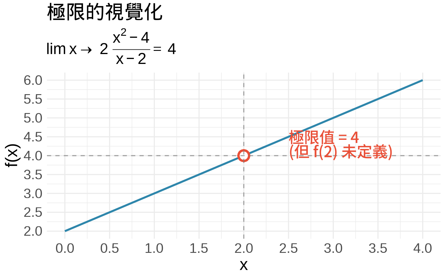
$$f(x) = \frac{x^2 - 4}{x - 2}$$
當 $x = 2$ 時,分子分母都是零,函數沒有定義。但是,當 $x$ **趨近** 2 時會發生什麼?
```{r}
#| label: fig-limit-basic
#| fig-cap: "極限的視覺化:當 x → 2 時,f(x) 趨近於 4"
#| fig-width: 8
#| fig-height: 5
# 建立資料
x <- seq(0, 4, by = 0.01)
x <- x[x != 2]  # 移除 x = 2

# 實際上 (x² - 4)/(x - 2) = (x-2)(x+2)/(x-2) = x + 2
f_x <- (x^2 - 4) / (x - 2)

df <- data.frame(x = x, y = f_x)

ggplot(df, aes(x, y)) +
  geom_line(color = "#2E86AB", linewidth = 1.2) +
  # 標記極限值
  geom_point(aes(x = 2, y = 4), shape = 21, size = 5,
             fill = "white", color = "#E94F37", stroke = 2) +
  # 虛線輔助線
  geom_hline(yintercept = 4, linetype = "dashed",
             color = "gray50", alpha = 0.7) +
  geom_vline(xintercept = 2, linetype = "dashed",
             color = "gray50", alpha = 0.7) +
  # 標註
  annotate("text", x = 2.5, y = 4.3,
           label = "極限值 = 4\n(但 f(2) 未定義)",
           hjust = 0, size = 4.5, color = "#E94F37") +
  labs(
    title = "極限的視覺化",
    subtitle = expression(lim(x %->% 2)~frac(x^2 - 4, x - 2) == 4),
    x = "x",
    y = "f(x)"
  ) +
  scale_x_continuous(breaks = seq(0, 4, 0.5)) +
  scale_y_continuous(breaks = seq(0, 6, 0.5)) +
  theme_minimal(base_size = 14) +
  theme(
    plot.title = element_text(face = "bold", size = 16),
    plot.subtitle = element_text(size = 13)
  )
```
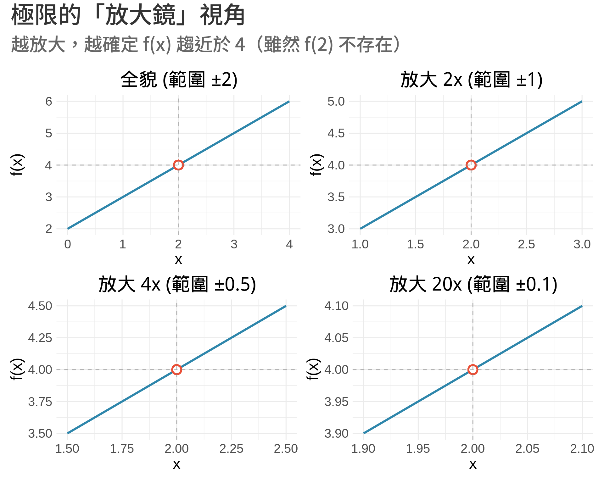
### 「放大鏡」效果:越靠近越清楚
要真正理解極限,我們可以用「放大鏡」的方式,越放越大,觀察 $x = 2$ 附近的行為。
```{r}
#| label: fig-limit-zoom
#| fig-cap: "放大鏡效果:越放大越確定 f(x) 趨近於 4"
#| fig-width: 10
#| fig-height: 8
# 建立四個不同放大程度的圖
create_zoom_plot <- function(x_center, x_range, zoom_label) {
  x_min <- x_center - x_range
  x_max <- x_center + x_range

  # 建立資料
  x_seq <- seq(x_min, x_max, length.out = 200)
  x_seq <- x_seq[abs(x_seq - 2) > 0.001]  # 避免除以零

  y_seq <- (x_seq^2 - 4) / (x_seq - 2)

  df_zoom <- data.frame(x = x_seq, y = y_seq)

  ggplot(df_zoom, aes(x, y)) +
    geom_line(color = "#2E86AB", linewidth = 1.2) +
    geom_point(aes(x = 2, y = 4), shape = 21, size = 4,
               fill = "white", color = "#E94F37", stroke = 1.5) +
    geom_hline(yintercept = 4, linetype = "dashed",
               color = "gray50", alpha = 0.5) +
    geom_vline(xintercept = 2, linetype = "dashed",
               color = "gray50", alpha = 0.5) +
    labs(
      title = zoom_label,
      x = "x",
      y = "f(x)"
    ) +
    coord_cartesian(
      xlim = c(x_min, x_max),
      ylim = c(4 - x_range, 4 + x_range)
    ) +
    theme_minimal(base_size = 12) +
    theme(
      plot.title = element_text(face = "bold", hjust = 0.5)
    )
}

# 建立四個不同放大程度
p1 <- create_zoom_plot(2, 2, "全貌 (範圍 ±2)")
p2 <- create_zoom_plot(2, 1, "放大 2x (範圍 ±1)")
p3 <- create_zoom_plot(2, 0.5, "放大 4x (範圍 ±0.5)")
p4 <- create_zoom_plot(2, 0.1, "放大 20x (範圍 ±0.1)")

# 組合圖形
(p1 | p2) / (p3 | p4) +
  plot_annotation(
    title = "極限的「放大鏡」視角",
    subtitle = "越放大,越確定 f(x) 趨近於 4(雖然 f(2) 不存在)",
    theme = theme(
      plot.title = element_text(size = 18, face = "bold"),
      plot.subtitle = element_text(size = 14)
    )
  )
```
### 數值驗證:逐步逼近
讓我們用數值來驗證極限:
```{r}
#| label: tbl-limit-numerical
#| tbl-cap: "從左側和右側逼近 x = 2"
# 從左側逼近
x_left <- 2 - c(1, 0.1, 0.01, 0.001, 0.0001)
f_left <- (x_left^2 - 4) / (x_left - 2)

# 從右側逼近
x_right <- 2 + c(1, 0.1, 0.01, 0.001, 0.0001)
f_right <- (x_right^2 - 4) / (x_right - 2)

# 建立表格
limit_table <- data.frame(
  `從左逼近 x` = x_left,
  `f(x) 值` = round(f_left, 6),
  `從右逼近 x` = x_right,
  `f(x) 值 ` = round(f_right, 6)
)

knitr::kable(limit_table, align = "c")
```
從表格可以清楚看到,無論從左或從右逼近 $x = 2$,函數值都趨近於 4。
## 數學定義
### 極限的嚴格定義
::: {.callout-note icon="false"}
## 極限的 ε-δ 定義
我們說 $\lim_{x \to a} f(x) = L$,如果:
對於任意小的 $\varepsilon > 0$,存在 $\delta > 0$,使得當 $0 < |x - a| < \delta$ 時,有 $|f(x) - L| < \varepsilon$。
**白話翻譯**:無論你要求 $f(x)$ 與 $L$ 有多接近($\varepsilon$ 有多小),我都能找到一個 $x$ 與 $a$ 的距離範圍($\delta$),讓在這範圍內的所有 $f(x)$ 都滿足你的要求。
:::
### 單側極限
- **右極限**:$\lim_{x \to a^+} f(x) = L$ 表示從右側($x > a$)趨近
- **左極限**:$\lim_{x \to a^-} f(x) = L$ 表示從左側($x < a$)趨近
::: {.callout-important}
## 極限存在的條件
極限 $\lim_{x \to a} f(x)$ 存在,當且僅當:
$$\lim_{x \to a^-} f(x) = \lim_{x \to a^+} f(x)$$
也就是說,左極限和右極限必須相等。
:::
### 極限的運算性質
假設 $\lim_{x \to a} f(x) = L$ 且 $\lim_{x \to a} g(x) = M$,則:
1. **和的極限**:$\lim_{x \to a} [f(x) + g(x)] = L + M$
2. **積的極限**:$\lim_{x \to a} [f(x) \cdot g(x)] = L \cdot M$
3. **商的極限**:$\lim_{x \to a} \frac{f(x)}{g(x)} = \frac{L}{M}$(若 $M \neq 0$)
## 練習題
### 觀念題
1. **判斷題**:如果 $f(a)$ 沒有定義,那麼 $\lim_{x \to a} f(x)$ 一定不存在。(O / X)
::: {.callout-tip collapse="true" title="參考答案"}
答案是 **X(錯誤)**。極限的存在與函數值是否有定義無關。本章的經典範例 $f(x) = \frac{x^2-4}{x-2}$ 就是最好的證明:雖然 $f(2)$ 未定義,但 $\lim_{x \to 2} f(x) = 4$ 是存在的。極限只關心函數在 $a$ 點**附近**的行為,而不是在 $a$ 點**本身**的值。
:::
2. **選擇題**:下列哪個敘述是正確的?
- (A) 極限存在,函數值一定存在
- (B) 函數值存在,極限一定存在
- (C) 極限值等於函數值
- (D) 以上皆非
::: {.callout-tip collapse="true" title="參考答案"}
答案是 **(D) 以上皆非**。選項 (A) 錯:極限存在不代表函數值存在(如 $\frac{x^2-4}{x-2}$ 在 $x=2$ 處)。選項 (B) 錯:函數值存在不保證極限存在(如分段函數在跳躍點)。選項 (C) 錯:極限值不一定等於函數值,下一章「連續性」會詳細討論這個條件。
:::
3. **問答題**:用自己的話解釋「左極限」與「右極限」的差異,並舉一個醫學例子。
::: {.callout-tip collapse="true" title="參考答案"}
**左極限**是從小於 $a$ 的方向趨近,**右極限**是從大於 $a$ 的方向趨近。醫學例子:藥物劑量-反應關係中,某些藥物存在「閾值效應」(threshold effect)。在閾值劑量之前(左側),反應幾乎為零;超過閾值後(右側),反應迅速上升。此時左極限和右極限不相等,極限不存在,代表在該劑量點有明顯的不連續性。
:::
### 計算題
4. 計算下列極限:
a. $\lim_{x \to 3} \frac{x^2 - 9}{x - 3}$
b. $\lim_{x \to 0} \frac{x^2 + 2x}{x}$
c. $\lim_{x \to 1} \frac{x^3 - 1}{x - 1}$
::: {.callout-tip collapse="true" title="參考答案"}
**a.** 因式分解:$\frac{x^2-9}{x-3} = \frac{(x-3)(x+3)}{x-3} = x+3$(當 $x \neq 3$),所以 $\lim_{x \to 3} (x+3) = 6$。
**b.** 提出 $x$:$\frac{x^2+2x}{x} = \frac{x(x+2)}{x} = x+2$(當 $x \neq 0$),所以 $\lim_{x \to 0} (x+2) = 2$。
**c.** 因式分解:$x^3-1 = (x-1)(x^2+x+1)$,所以 $\frac{x^3-1}{x-1} = x^2+x+1$(當 $x \neq 1$),因此 $\lim_{x \to 1} (x^2+x+1) = 3$。
:::
5. 考慮函數:
$$f(x) = \begin{cases}
x + 1 & \text{if } x < 2 \\
5 & \text{if } x = 2 \\
2x - 1 & \text{if } x > 2
\end{cases}$$
求:(a) $\lim_{x \to 2^-} f(x)$, (b) $\lim_{x \to 2^+} f(x)$, (c) $\lim_{x \to 2} f(x)$ 是否存在?
::: {.callout-tip collapse="true" title="參考答案"}
**(a)** 從左側趨近:使用 $x < 2$ 的公式 $f(x) = x + 1$,所以 $\lim_{x \to 2^-} f(x) = 2 + 1 = 3$。
**(b)** 從右側趨近:使用 $x > 2$ 的公式 $f(x) = 2x - 1$,所以 $\lim_{x \to 2^+} f(x) = 2(2) - 1 = 3$。
**(c)** 因為左極限 = 右極限 = 3,所以 $\lim_{x \to 2} f(x) = 3$ **存在**。注意:極限值是 3,但 $f(2) = 5$,所以極限值 ≠ 函數值。
:::
### R 操作題
6. **視覺化練習**:修改以下程式碼,視覺化 $\lim_{x \to 0} \frac{\sin(x)}{x}$ 的極限(提示:極限值是 1)
```r
x <- seq(-0.5, 0.5, by = 0.001)
x <- x[x != 0]

f_x <- sin(x) / x

df <- data.frame(x = x, y = f_x)

ggplot(df, aes(x, y)) +
  geom_line(color = "#2E86AB", linewidth = 1.2) +
  geom_hline(yintercept = ___, linetype = "dashed", color = "#E94F37") +
  labs(title = "sin(x)/x 的極限")
```
::: {.callout-tip collapse="true" title="參考答案"}
填入 `yintercept = 1`。執行程式碼後,你會看到函數曲線在 $x = 0$ 附近無限接近 1。這個極限是微積分中的重要極限之一,在三角函數的微分公式推導中扮演關鍵角色。紅色虛線($y = 1$)清楚顯示極限值的位置。
:::
7. **數值實驗**:建立一個表格,驗證 $\lim_{x \to 0} \frac{e^x - 1}{x} = 1$
::: {.callout-tip collapse="true" title="參考答案"}
參考本章「數值驗證」的表格程式碼,從左右兩側逼近 $x = 0$。範例程式:
```r
x_left <- -c(0.1, 0.01, 0.001, 0.0001)
f_left <- (exp(x_left) - 1) / x_left
x_right <- c(0.1, 0.01, 0.001, 0.0001)
f_right <- (exp(x_right) - 1) / x_right
```
你會發現當 $x$ 越接近 0,函數值越接近 1。這個極限是指數函數微分的基礎:$\frac{d}{dx}e^x = e^x$ 的證明核心。
:::
## 統計應用
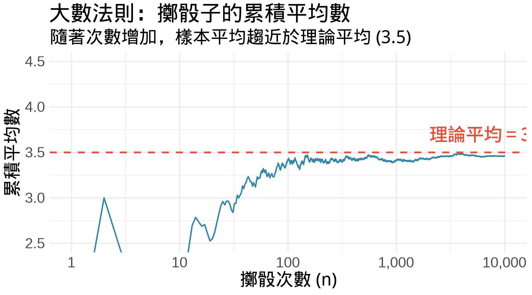
### 大數法則 (Law of Large Numbers)
極限在統計學中最重要的應用之一是**大數法則** [@dekking2005modern]:
> 當樣本數 $n$ 趨近於無窮大時,樣本平均數 $\bar{X}_n$ 會趨近於母體平均數 $\mu$
數學表達:
$$\lim_{n \to \infty} \bar{X}_n = \mu$$
```{r}
#| label: fig-law-of-large-numbers
#| fig-cap: "大數法則的視覺化:擲骰子實驗"
#| fig-width: 9
#| fig-height: 5
set.seed(42)

# 模擬擲骰子 10000 次
n_rolls <- 10000
dice_rolls <- sample(1:6, n_rolls, replace = TRUE)

# 計算累積平均數
cumulative_mean <- cumsum(dice_rolls) / seq_along(dice_rolls)

df_lln <- data.frame(
  n = 1:n_rolls,
  mean = cumulative_mean
)

ggplot(df_lln, aes(n, mean)) +
  geom_line(color = "#2E86AB", linewidth = 0.8) +
  geom_hline(yintercept = 3.5, linetype = "dashed",
             color = "#E94F37", linewidth = 1) +
  annotate("text", x = 7000, y = 3.7,
           label = "理論平均 = 3.5",
           color = "#E94F37", size = 5) +
  labs(
    title = "大數法則:擲骰子的累積平均數",
    subtitle = "隨著次數增加,樣本平均趨近於理論平均 (3.5)",
    x = "擲骰次數 (n)",
    y = "累積平均數"
  ) +
  scale_x_log10(labels = scales::comma) +
  coord_cartesian(ylim = c(2.5, 4.5)) +
  theme_minimal(base_size = 14) +
  theme(
    plot.title = element_text(face = "bold")
  )
```
### 連續機率分布的定義
連續型隨機變數的機率密度函數 (PDF) 必須滿足 [@rice2006mathematical]:
$$\int_{-\infty}^{\infty} f(x) dx = 1$$
這個積分的定義就建立在極限之上:
$$\int_{-\infty}^{\infty} f(x) dx = \lim_{a \to -\infty} \lim_{b \to \infty} \int_a^b f(x) dx$$
### P-value 的極端情況
在假設檢定中,p-value 本質上是計算「極端情況」的機率 [@lehmann2005testing]:
$$p\text{-value} = P(|T| \geq |t_{\text{obs}}|)$$
當檢定統計量 $t$ 趨近於無窮大時:
$$\lim_{t \to \infty} P(|T| \geq t) = 0$$
這解釋了為什麼極端的檢定統計量會給出非常小的 p-value。
## 本章重點整理 {.unnumbered}
::: {.callout-tip icon="false"}
## 核心概念
1. **極限是「趨近」而非「等於」**:$\lim_{x \to a} f(x) = L$ 不代表 $f(a) = L$
2. **極限存在與函數值無關**:$f(a)$ 可以不存在,但極限仍可存在
3. **左右極限必須相等**:$\lim_{x \to a^-} f(x) = \lim_{x \to a^+} f(x)$ 才能說極限存在
4. **統計應用**:
- 大數法則:樣本平均趨近母體平均
- 連續分布的定義基礎
- 理解極端事件的機率
5. **視覺化理解**:用「放大鏡」的概念,越靠近越清楚函數的行為
:::
::: {.callout-note}
## 下一章預告
在理解了極限的概念後,我們將學習**連續性**:什麼樣的函數可以「一筆畫完」?這對於理解機率密度函數 (PDF) 至關重要。
:::