---
title: "Chapter 10: 瑕積分"
---
```{r}
#| include: false
source(here::here("R/_common.R"))
```
## 學習目標 {.unnumbered}
- 理解瑕積分 (Improper Integrals) 的定義
- 處理積分範圍延伸到無窮大的情況
- 理解為什麼機率密度函數必須滿足總面積等於 1
- 掌握收斂與發散的概念
- 應用瑕積分於統計:期望值、存活函數
## 什麼是瑕積分?
在前面的章節,我們處理的都是**有限區間**的積分:$\int_a^b f(x)dx$,其中 $a, b$ 都是有限數值。
但在統計學中,我們經常遇到 [@stewart2015calculus; @wackerly2008mathematical]:
- 積分範圍到**無窮大**:$\int_0^{\infty} f(x)dx$
- 積分範圍從**負無窮到正無窮**:$\int_{-\infty}^{\infty} f(x)dx$
這些叫做 **瑕積分 (Improper Integrals)**。
### 為什麼統計需要瑕積分?
1. **機率密度函數的正規化**:
$$\int_{-\infty}^{\infty} f(x)dx = 1$$
2. **期望值的計算**:
$$E(X) = \int_{-\infty}^{\infty} x \cdot f(x)dx$$
3. **存活函數**:
$$S(t) = P(T > t) = \int_t^{\infty} f(x)dx$$
4. **累積風險函數**:
$$H(t) = \int_0^t h(u)du$$
## 瑕積分的定義
### 上界為無窮大
$$\int_a^{\infty} f(x)dx = \lim_{b \to \infty} \int_a^b f(x)dx$$
**步驟**:
1. 先計算有限區間的積分
2. 讓上界趨近無窮大
3. 看極限是否存在
### 下界為負無窮大
$$\int_{-\infty}^b f(x)dx = \lim_{a \to -\infty} \int_a^b f(x)dx$$
### 雙邊無窮大
$$\int_{-\infty}^{\infty} f(x)dx = \lim_{a \to -\infty} \int_a^0 f(x)dx + \lim_{b \to \infty} \int_0^b f(x)dx$$
## 收斂與發散
**收斂 (Convergent)**:極限存在且為有限值
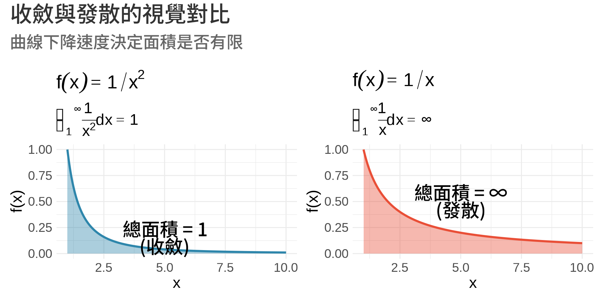
$$\int_1^{\infty} \frac{1}{x^2}dx = \lim_{b \to \infty} \left[-\frac{1}{x}\right]_1^b = 1$$
**發散 (Divergent)**:極限不存在或為無窮大
$$\int_1^{\infty} \frac{1}{x}dx = \lim_{b \to \infty} \left[\ln x\right]_1^b = \infty$$
### 視覺化比較
```{r}
#| label: fig-convergence-comparison
#| fig-cap: "收斂與發散的視覺對比"
#| warning: false
#| message: false
#| fig-width: 10
#| fig-height: 5
x <- seq(1, 10, by = 0.01)

# 1/x² (收斂)
y1 <- 1 / x^2

p1 <- ggplot(data.frame(x, y = y1), aes(x, y)) +
  geom_area(fill = "#2E86AB", alpha = 0.4) +
  geom_line(linewidth = 1.2, color = "#2E86AB") +
  annotate("text", x = 5, y = 0.15,
           label = "總面積 = 1\n(收斂)",
           size = 5, fontface = "bold") +
  labs(
    title = expression(f(x) == 1/x^2),
    subtitle = expression(integral(frac(1, x^2)*dx, 1, infinity) == 1),
    x = "x", y = "f(x)"
  ) +
  coord_cartesian(ylim = c(0, 1)) +
  theme_minimal(base_size = 12)

# 1/x (發散)
y2 <- 1 / x

p2 <- ggplot(data.frame(x, y = y2), aes(x, y)) +
  geom_area(fill = "#E94F37", alpha = 0.4) +
  geom_line(linewidth = 1.2, color = "#E94F37") +
  annotate("text", x = 5, y = 0.5,
           label = "總面積 = ∞\n(發散)",
           size = 5, fontface = "bold") +
  labs(
    title = expression(f(x) == 1/x),
    subtitle = expression(integral(frac(1, x)*dx, 1, infinity) == infinity),
    x = "x", y = "f(x)"
  ) +
  coord_cartesian(ylim = c(0, 1)) +
  theme_minimal(base_size = 12)

p1 + p2 +
  plot_annotation(
    title = "收斂與發散的視覺對比",
    subtitle = "曲線下降速度決定面積是否有限"
  )
```
**關鍵觀察**:
- $\frac{1}{x^2}$ 下降得夠快 → 面積收斂
- $\frac{1}{x}$ 下降得不夠快 → 面積發散
## 統計應用 I:機率密度函數的正規化
### 為什麼總面積必須等於 1?
對於任意機率密度函數 $f(x)$ [@casella2002statistical; @degroot2012probability]:
$$\int_{-\infty}^{\infty} f(x)dx = 1$$
**原因**:機率的總和必須是 100%。
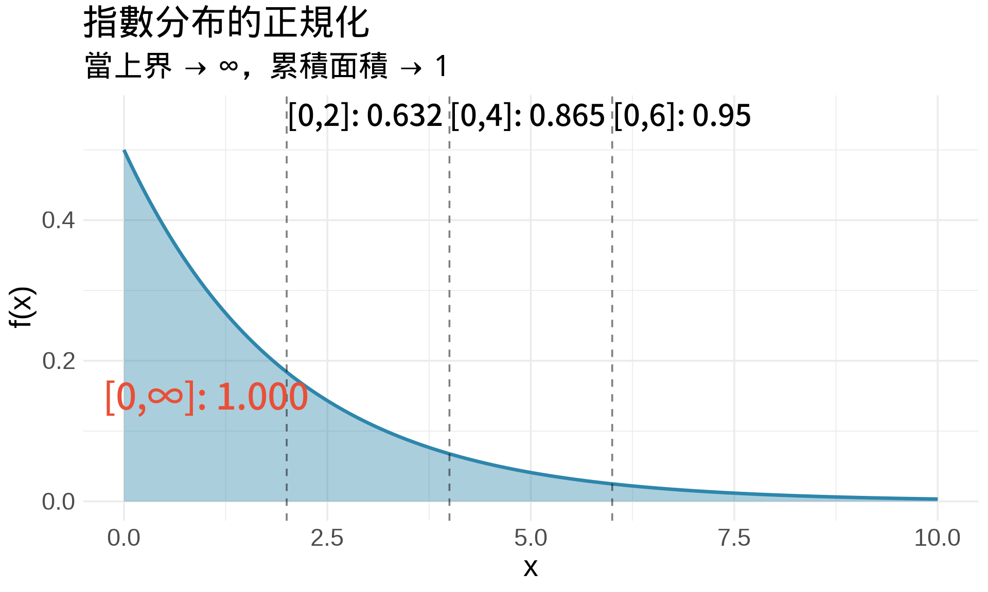
### 範例:指數分布
**指數分布**:$f(x) = \lambda e^{-\lambda x}$,$x \geq 0$
**驗證總面積 = 1**:
$$\int_0^{\infty} \lambda e^{-\lambda x}dx = \lim_{b \to \infty} \left[-e^{-\lambda x}\right]_0^b$$
$$= \lim_{b \to \infty} \left(-e^{-\lambda b} + 1\right) = 0 + 1 = 1$$
✅ 收斂,且總面積 = 1!
```{r}
#| label: fig-exponential-normalization
#| fig-cap: "指數分布的正規化"
#| warning: false
#| message: false
lambda <- 0.5
x <- seq(0, 10, by = 0.01)
y <- lambda * exp(-lambda * x)

# 計算不同上界的累積面積
upper_bounds <- c(2, 4, 6, 10, 20)
areas <- sapply(upper_bounds, function(b) {
  integrate(function(x) lambda * exp(-lambda * x), lower = 0, upper = b)$value
})

ggplot(data.frame(x, y), aes(x, y)) +
  geom_area(fill = "#2E86AB", alpha = 0.4) +
  geom_line(linewidth = 1.2, color = "#2E86AB") +
  # 標記幾個累積面積
  geom_vline(xintercept = c(2, 4, 6), linetype = "dashed", alpha = 0.5) +
  annotate("text", x = 2, y = lambda + 0.05,
           label = paste0("[0,2]: ", round(areas[1], 3)), hjust = 0) +
  annotate("text", x = 4, y = lambda + 0.05,
           label = paste0("[0,4]: ", round(areas[2], 3)), hjust = 0) +
  annotate("text", x = 6, y = lambda + 0.05,
           label = paste0("[0,6]: ", round(areas[3], 3)), hjust = 0) +
  annotate("text", x = 1, y = 0.15,
           label = "[0,∞]: 1.000",
           size = 6, fontface = "bold", color = "#E94F37") +
  labs(
    title = "指數分布的正規化",
    subtitle = expression("當上界 → ∞,累積面積 → 1"),
    x = "x", y = "f(x)"
  ) +
  theme_minimal(base_size = 14)
```
**R 驗證**:
```{r}
# 不同上界的面積
lambda <- 0.5
f <- function(x) lambda * exp(-lambda * x)

cat("積分到 10:", integrate(f, 0, 10)$value, "\n")
cat("積分到 20:", integrate(f, 0, 20)$value, "\n")
cat("積分到 50:", integrate(f, 0, 50)$value, "\n")
cat("積分到 ∞:", integrate(f, 0, Inf)$value, "\n")
```
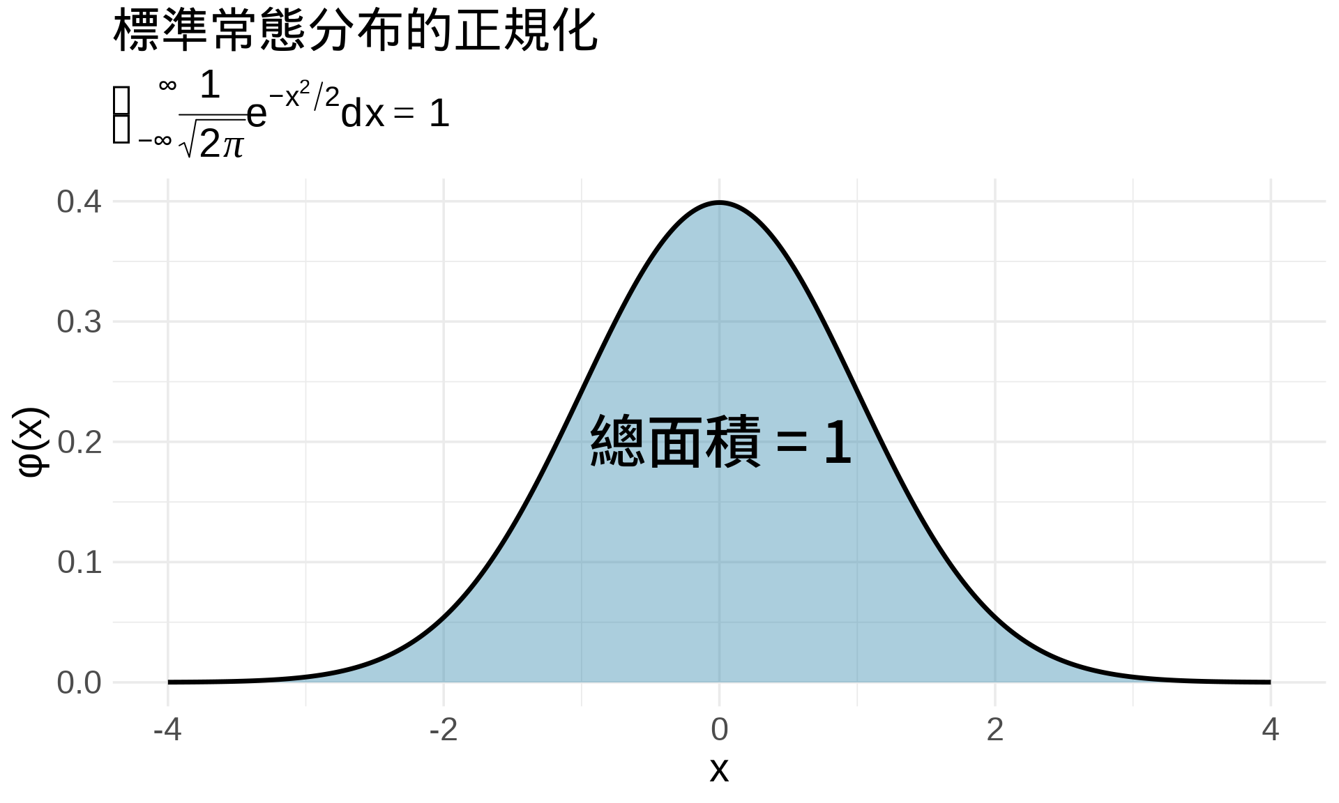
### 範例:常態分布
**標準常態分布**:$f(x) = \frac{1}{\sqrt{2\pi}}e^{-x^2/2}$
**驗證**:
$$\int_{-\infty}^{\infty} \frac{1}{\sqrt{2\pi}}e^{-x^2/2}dx = 1$$
這個積分**無法用初等函數表達**,但可以用數值方法驗證:
```{r}
# R 驗證
f <- function(x) dnorm(x)
area <- integrate(f, lower = -Inf, upper = Inf)$value

cat("總面積:", round(area, 10), "\n")
cat("理論值:", 1, "\n")
```
**視覺化**:
```{r}
#| label: fig-normal-normalization
#| fig-cap: "常態分布的總面積 = 1"
#| warning: false
#| message: false
x <- seq(-4, 4, by = 0.01)
y <- dnorm(x)

ggplot(data.frame(x, y), aes(x, y)) +
  geom_area(fill = "#2E86AB", alpha = 0.4) +
  geom_line(linewidth = 1.2, color = "black") +
  annotate("text", x = 0, y = 0.2,
           label = "總面積 = 1",
           size = 7, fontface = "bold") +
  labs(
    title = "標準常態分布的正規化",
    subtitle = expression(integral(frac(1, sqrt(2*pi))*e^{-x^2/2}*dx, -infinity, infinity) == 1),
    x = "x", y = "φ(x)"
  ) +
  theme_minimal(base_size = 14)
```
## 統計應用 II:期望值的計算
### 無窮範圍的期望值
對於 $X \geq 0$ 的隨機變數:
$$E(X) = \int_0^{\infty} x \cdot f(x)dx$$
這也是一個瑕積分!
### 範例:指數分布的期望值
**指數分布**:$f(x) = \lambda e^{-\lambda x}$
**計算**:
$$E(X) = \int_0^{\infty} x \cdot \lambda e^{-\lambda x}dx$$
用分部積分法(令 $u = x$, $dv = \lambda e^{-\lambda x}dx$):
$$= \left[-xe^{-\lambda x}\right]_0^{\infty} + \int_0^{\infty} e^{-\lambda x}dx$$
$$= 0 + \frac{1}{\lambda} = \frac{1}{\lambda}$$
**R 驗證**:
```{r}
# 數值積分
lambda <- 2
f <- function(x) x * lambda * exp(-lambda * x)
expectation <- integrate(f, lower = 0, upper = Inf)$value

cat("數值積分:", round(expectation, 5), "\n")
cat("理論值 1/λ:", 1/lambda, "\n")
# 用模擬驗證
set.seed(42)
x <- rexp(100000, rate = lambda)
cat("模擬平均:", round(mean(x), 5), "\n")
```
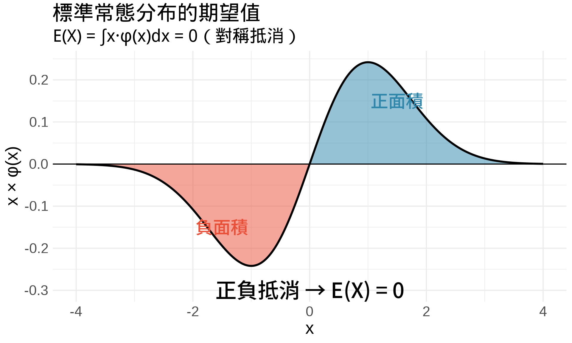
### 範例:常態分布的期望值
**標準常態分布**:
$$E(X) = \int_{-\infty}^{\infty} x \cdot \frac{1}{\sqrt{2\pi}}e^{-x^2/2}dx = 0$$
**為什麼是 0?**
因為函數 $x \cdot f(x)$ 是**奇函數** (odd function),對稱於原點,正負抵消:
```{r}
#| label: fig-normal-expectation
#| fig-cap: "常態分布期望值:對稱抵消"
#| warning: false
#| message: false
x <- seq(-4, 4, by = 0.01)
y <- x * dnorm(x)  # x * f(x)

df <- data.frame(x, y)
df_pos <- df[df$y >= 0, ]
df_neg <- df[df$y < 0, ]

ggplot() +
  geom_area(data = df_pos, aes(x, y), fill = "#2E86AB", alpha = 0.5) +
  geom_area(data = df_neg, aes(x, y), fill = "#E94F37", alpha = 0.5) +
  geom_line(data = df, aes(x, y), linewidth = 1.2) +
  geom_hline(yintercept = 0, color = "black") +
  annotate("text", x = 1.5, y = 0.15, label = "正面積", color = "#2E86AB", size = 5) +
  annotate("text", x = -1.5, y = -0.15, label = "負面積", color = "#E94F37", size = 5) +
  annotate("text", x = 0, y = -0.3,
           label = "正負抵消 → E(X) = 0",
           size = 6, fontface = "bold") +
  labs(
    title = "標準常態分布的期望值",
    subtitle = "E(X) = ∫x·φ(x)dx = 0(對稱抵消)",
    x = "x", y = "x × φ(x)"
  ) +
  theme_minimal(base_size = 14)
```
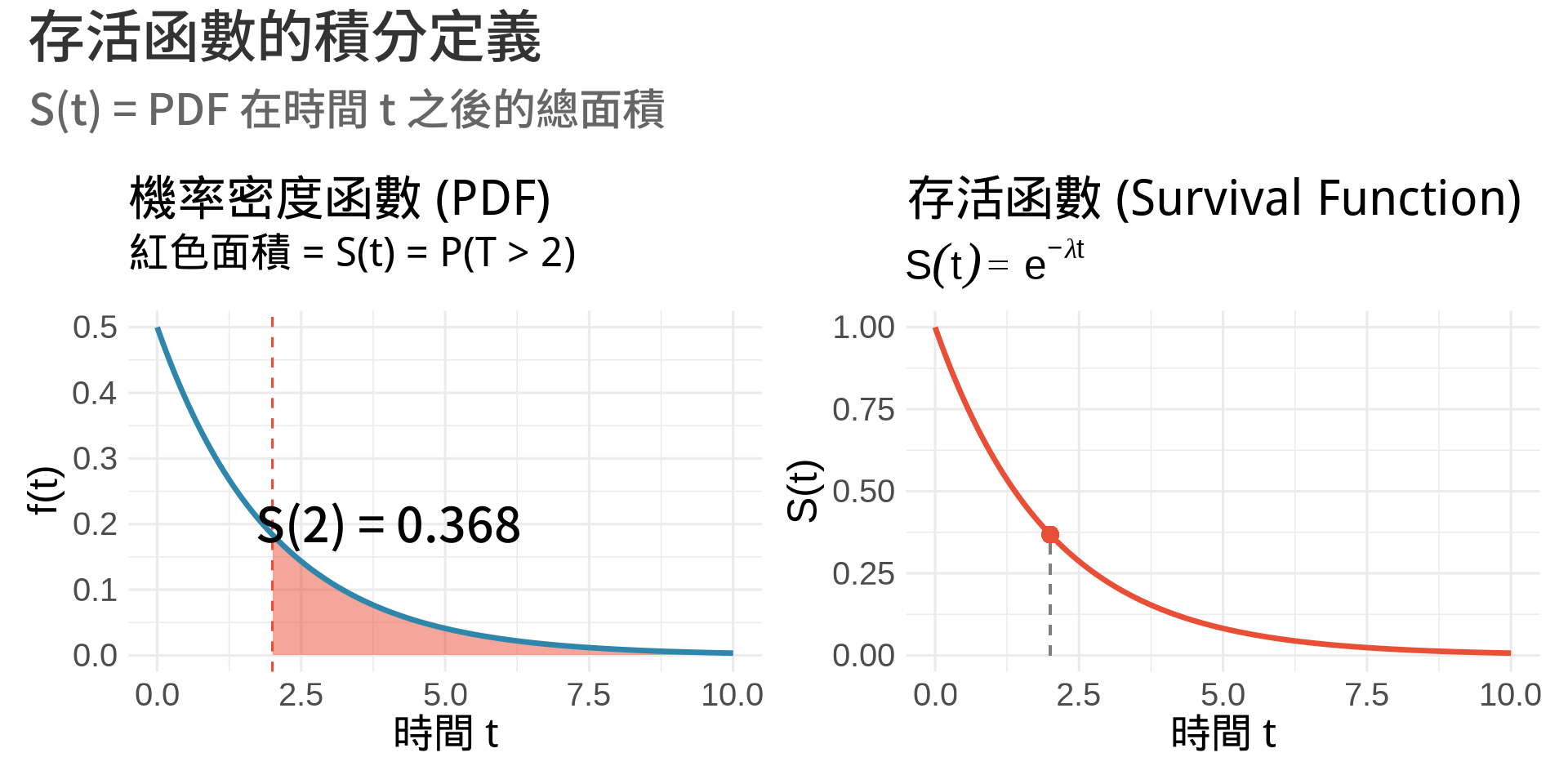
## 統計應用 III:存活函數
### 定義
**存活函數 (Survival Function)** [@collett2015modelling; @klein2003survival]:
$$S(t) = P(T > t) = \int_t^{\infty} f(x)dx$$
表示「存活超過時間 $t$」的機率。
### 視覺化:指數分布的存活函數
```{r}
#| label: fig-survival-function
#| fig-cap: "存活函數:時間 t 之後的面積"
#| warning: false
#| message: false
#| fig-width: 10
#| fig-height: 5
lambda <- 0.5
x <- seq(0, 10, by = 0.01)
f_x <- lambda * exp(-lambda * x)

# 在 t = 2 的存活區域
t0 <- 2
x_survive <- x[x >= t0]
f_survive <- lambda * exp(-lambda * x_survive)

p1 <- ggplot(data.frame(x, y = f_x), aes(x, y)) +
  geom_area(data = data.frame(x = x_survive, y = f_survive),
            aes(x, y), fill = "#E94F37", alpha = 0.5) +
  geom_line(linewidth = 1.2, color = "#2E86AB") +
  geom_vline(xintercept = t0, linetype = "dashed", color = "#E94F37") +
  annotate("text", x = 4, y = 0.2,
           label = paste0("S(2) = ", round(exp(-lambda * t0), 3)),
           size = 5, fontface = "bold") +
  labs(
    title = "機率密度函數 (PDF)",
    subtitle = "紅色面積 = S(t) = P(T > 2)",
    x = "時間 t", y = "f(t)"
  ) +
  theme_minimal(base_size = 12)

# 存活函數曲線
t <- seq(0, 10, by = 0.01)
S_t <- exp(-lambda * t)  # 指數分布的存活函數

p2 <- ggplot(data.frame(t, S_t), aes(t, S_t)) +
  geom_line(color = "#E94F37", linewidth = 1.2) +
  geom_point(aes(x = t0, y = exp(-lambda * t0)),
             size = 3, color = "#E94F37") +
  geom_segment(aes(x = t0, xend = t0, y = 0, yend = exp(-lambda * t0)),
               linetype = "dashed", color = "gray50") +
  labs(
    title = "存活函數 (Survival Function)",
    subtitle = expression(S(t) == e^{-lambda*t}),
    x = "時間 t", y = "S(t)"
  ) +
  theme_minimal(base_size = 12)

p1 + p2 +
  plot_annotation(
    title = "存活函數的積分定義",
    subtitle = "S(t) = PDF 在時間 t 之後的總面積"
  )
```
**R 計算**:
```{r}
lambda <- 0.5
t <- 2

# 方法 1:用存活函數公式
S_formula <- exp(-lambda * t)

# 方法 2:用積分
f <- function(x) lambda * exp(-lambda * x)
S_integrate <- integrate(f, lower = t, upper = Inf)$value

# 方法 3:用 R 的 pexp()
S_pexp <- 1 - pexp(t, rate = lambda)

cat("公式計算:", round(S_formula, 5), "\n")
cat("積分計算:", round(S_integrate, 5), "\n")
cat("pexp 計算:", round(S_pexp, 5), "\n")
```
### 醫學意義
在**存活分析 (Survival Analysis)** 中 [@collett2015modelling; @klein2003survival]:
- $S(t)$:病患在時間 $t$ 仍存活的機率
- $h(t)$:hazard function,瞬時死亡風險
- 關係:$S(t) = \exp\left(-\int_0^t h(u)du\right)$
## 收斂判斷原則
### 比較判別法
如果 $0 \leq f(x) \leq g(x)$:
- $\int_a^{\infty} g(x)dx$ 收斂 → $\int_a^{\infty} f(x)dx$ 收斂
- $\int_a^{\infty} f(x)dx$ 發散 → $\int_a^{\infty} g(x)dx$ 發散
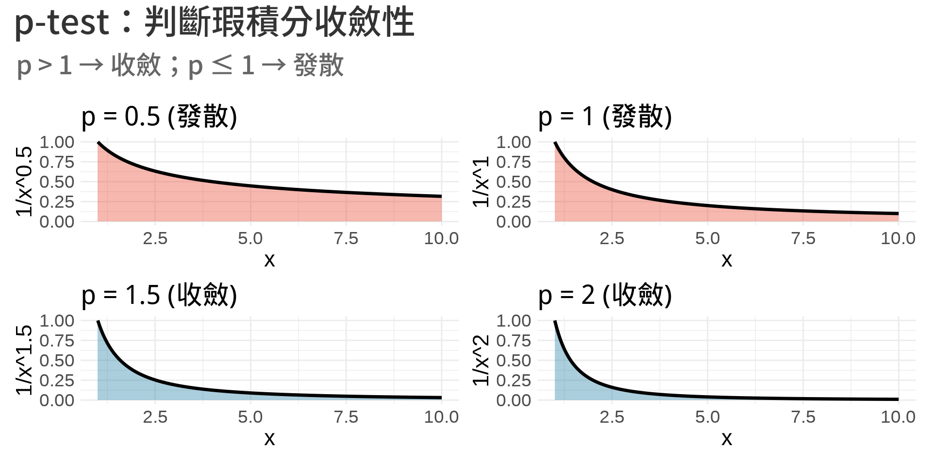
### p-test for integrals
$$\int_1^{\infty} \frac{1}{x^p}dx \begin{cases}
\text{收斂} & \text{if } p > 1 \\
\text{發散} & \text{if } p \leq 1
\end{cases}$$
**視覺化**:
```{r}
#| label: fig-p-test
#| fig-cap: "p-test:不同 p 值的收斂性"
#| warning: false
#| message: false
#| fig-width: 10
#| fig-height: 5
x <- seq(1, 10, by = 0.01)

create_p_plot <- function(p_val, status) {
  y <- 1 / x^p_val

  ggplot(data.frame(x, y), aes(x, y)) +
    geom_area(fill = ifelse(status == "收斂", "#2E86AB", "#E94F37"),
              alpha = 0.4) +
    geom_line(linewidth = 1.2, color = "black") +
    labs(
      title = paste0("p = ", p_val, " (", status, ")"),
      x = "x", y = paste0("1/x^", p_val)
    ) +
    coord_cartesian(ylim = c(0, 1)) +
    theme_minimal(base_size = 11)
}

p1 <- create_p_plot(0.5, "發散")
p2 <- create_p_plot(1, "發散")
p3 <- create_p_plot(1.5, "收斂")
p4 <- create_p_plot(2, "收斂")

(p1 | p2) / (p3 | p4) +
  plot_annotation(
    title = "p-test:判斷瑕積分收斂性",
    subtitle = "p > 1 → 收斂;p ≤ 1 → 發散"
  )
```
## 練習題
### 觀念題
1. 為什麼所有的機率密度函數都必須滿足 $\int_{-\infty}^{\infty} f(x)dx = 1$?
::: {.callout-tip collapse="true" title="參考答案"}
因為機率密度函數描述的是機率的分布,而所有可能結果的機率總和必須是 100%(即 1)。這個積分代表「所有可能的 x 值」發生的總機率,根據機率公理必須等於 1。如果不等於 1,就不是合法的機率分布。
:::
2. 說明「收斂」與「發散」的差別。
::: {.callout-tip collapse="true" title="參考答案"}
收斂 (Convergent) 表示瑕積分的極限存在且為有限值,意味著即使積分範圍延伸到無窮大,曲線下的總面積仍是有限的。發散 (Divergent) 則表示極限不存在或為無窮大,代表總面積是無限的。例如:$\int_1^{\infty} \frac{1}{x^2}dx = 1$(收斂),但 $\int_1^{\infty} \frac{1}{x}dx = \infty$(發散)。
:::
3. 為什麼 $\int_1^{\infty} \frac{1}{x}dx$ 發散,但 $\int_1^{\infty} \frac{1}{x^2}dx$ 收斂?
::: {.callout-tip collapse="true" title="參考答案"}
關鍵在於函數下降的速度。$\frac{1}{x^2}$ 下降得比 $\frac{1}{x}$ 快得多,使得其尾端面積快速縮小到可忽略。根據 p-test,$\int_1^{\infty} \frac{1}{x^p}dx$ 只有在 $p > 1$ 時才收斂。當 $p=1$ 時函數下降得不夠快,導致面積累積到無窮大;而 $p=2$ 時下降夠快,總面積收斂到 1。
:::
### 計算題
4. 判斷下列瑕積分是否收斂,若收斂則計算其值:
a. $\int_0^{\infty} e^{-x}dx$
b. $\int_1^{\infty} \frac{1}{x^3}dx$
c. $\int_0^{\infty} \frac{1}{1+x^2}dx$
```{r}
#| eval: false
# 提示
integrate(function(x) exp(-x), lower = 0, upper = Inf)
```
::: {.callout-tip collapse="true" title="參考答案"}
**a.** 收斂,值為 1。計算:$\int_0^{\infty} e^{-x}dx = \lim_{b \to \infty} [-e^{-x}]_0^b = \lim_{b \to \infty} (-e^{-b} + 1) = 1$
**b.** 收斂,值為 1/2。計算:$\int_1^{\infty} \frac{1}{x^3}dx = \lim_{b \to \infty} [-\frac{1}{2x^2}]_1^b = \lim_{b \to \infty} (-\frac{1}{2b^2} + \frac{1}{2}) = \frac{1}{2}$
**c.** 收斂,值為 $\pi/2$。這是 $\arctan(x)$ 的導數,所以 $\int_0^{\infty} \frac{1}{1+x^2}dx = \lim_{b \to \infty} [\arctan(x)]_0^b = \frac{\pi}{2} - 0 = \frac{\pi}{2}$
可用 R 驗證:`integrate(function(x) 1/(1+x^2), 0, Inf)$value` 約為 1.571(即 $\pi/2$)
:::
5. 驗證 Gamma 分布 $f(x) = \frac{\lambda^\alpha}{\Gamma(\alpha)} x^{\alpha-1} e^{-\lambda x}$ 的總面積是否為 1(用 R,設 $\alpha = 2$, $\lambda = 1$)。
::: {.callout-tip collapse="true" title="參考答案"}
```r
alpha <- 2
lambda <- 1
f <- function(x) dgamma(x, shape = alpha, rate = lambda)
area <- integrate(f, lower = 0, upper = Inf)$value
# area 應該等於 1.000000

# 或直接用公式
f_manual <- function(x) {
  (lambda^alpha / gamma(alpha)) * x^(alpha-1) * exp(-lambda * x)
}
integrate(f_manual, 0, Inf)$value  # 也是 1
```
結果確實為 1,驗證了 Gamma 分布是合法的機率密度函數。
:::
### R 操作題
6. 計算 Cauchy 分布的期望值:
$$E(X) = \int_{-\infty}^{\infty} x \cdot \frac{1}{\pi(1+x^2)}dx$$
會發生什麼事?為什麼?
```{r}
#| eval: false
f <- function(x) x * dcauchy(x)
integrate(f, lower = -Inf, upper = Inf)
```
::: {.callout-tip collapse="true" title="參考答案"}
R 會回報錯誤或警告訊息,因為這個積分**不收斂**(發散)!Cauchy 分布是一個特殊的例子,雖然它是合法的機率分布(總面積 = 1),但它的期望值不存在。原因是 $\frac{x}{1+x^2}$ 在尾端下降得不夠快,導致 $\int x \cdot f(x)dx$ 發散。這告訴我們:即使是合法的機率分布,也可能沒有有限的期望值!這在統計學中是很重要的反例。
:::
7. 繪製 Weibull 分布的存活函數:
$$S(t) = \exp\left(-\left(\frac{t}{\lambda}\right)^k\right)$$
設 $\lambda = 2$, $k = 1.5$,並標記中位存活時間($S(t) = 0.5$ 的點)。
```{r}
#| eval: false
pweibull(t, shape = k, scale = lambda, lower.tail = FALSE) # S(t)
```
::: {.callout-tip collapse="true" title="參考答案"}
```r
library(ggplot2)

lambda <- 2
k <- 1.5

# 中位存活時間:解 S(t) = 0.5
median_time <- lambda * (-log(0.5))^(1/k)  # ≈ 1.637

t <- seq(0, 6, by = 0.01)
S_t <- pweibull(t, shape = k, scale = lambda, lower.tail = FALSE)

ggplot(data.frame(t, S_t), aes(t, S_t)) +
  geom_line(color = "#2E86AB", linewidth = 1.2) +
  geom_hline(yintercept = 0.5, linetype = "dashed", color = "gray50") +
  geom_vline(xintercept = median_time, linetype = "dashed", color = "#E94F37") +
  geom_point(aes(x = median_time, y = 0.5), color = "#E94F37", size = 3) +
  annotate("text", x = median_time + 0.3, y = 0.5,
           label = paste0("中位存活時間 = ", round(median_time, 2)), hjust = 0) +
  labs(title = "Weibull 存活函數", x = "時間 t", y = "S(t)") +
  theme_minimal()
```
:::
## 本章重點整理 {.unnumbered}
1. **瑕積分**:積分範圍延伸到無窮大
2. **收斂與發散**:極限存在 versus 極限為無窮
3. **統計應用**:
- PDF 正規化:$\int_{-\infty}^{\infty} f(x)dx = 1$
- 期望值:$E(X) = \int_{-\infty}^{\infty} x \cdot f(x)dx$
- 存活函數:$S(t) = \int_t^{\infty} f(x)dx$
4. **p-test**:$\int_1^{\infty} \frac{1}{x^p}dx$ 在 $p > 1$ 時收斂
5. R 函數:`integrate(f, lower = -Inf, upper = Inf)` 處理無窮積分
---
**Part III 總結**:我們已經掌握了積分的三大主題:概念、計算技巧、無窮積分。這些是理解所有連續型機率分布的數學基礎!
**下一步**:在 Part IV,我們將進入**多變量微積分**,處理有多個變數的函數,這是理解多元統計方法的關鍵。