# 微分規則 (Differentiation Rules)
```{r}
#| include: false
source(here::here("R/_common.R"))
```
## 學習目標 {.unnumbered}
- 掌握基本微分規則:冪次、和差、乘法、除法
- 理解**連鎖律 (Chain Rule)** 的重要性
- 視覺化函數與其導數的關係
- 連結醫學統計:logit 函數的微分、PDF 與 CDF 的關係
## 為什麼需要微分規則?
上一章我們學了導數的定義:
$$
f'(x) = \lim_{h \to 0} \frac{f(x+h) - f(x)}{h}
$$
但每次都用定義計算太麻煩了!幸好數學家已經推導出一套**微分規則**,讓我們可以快速計算常見函數的導數。
就像開車:你可以理解引擎的運作原理(導數定義),但日常駕駛時只需要知道如何操作方向盤和油門(微分規則)。
## 基本微分規則
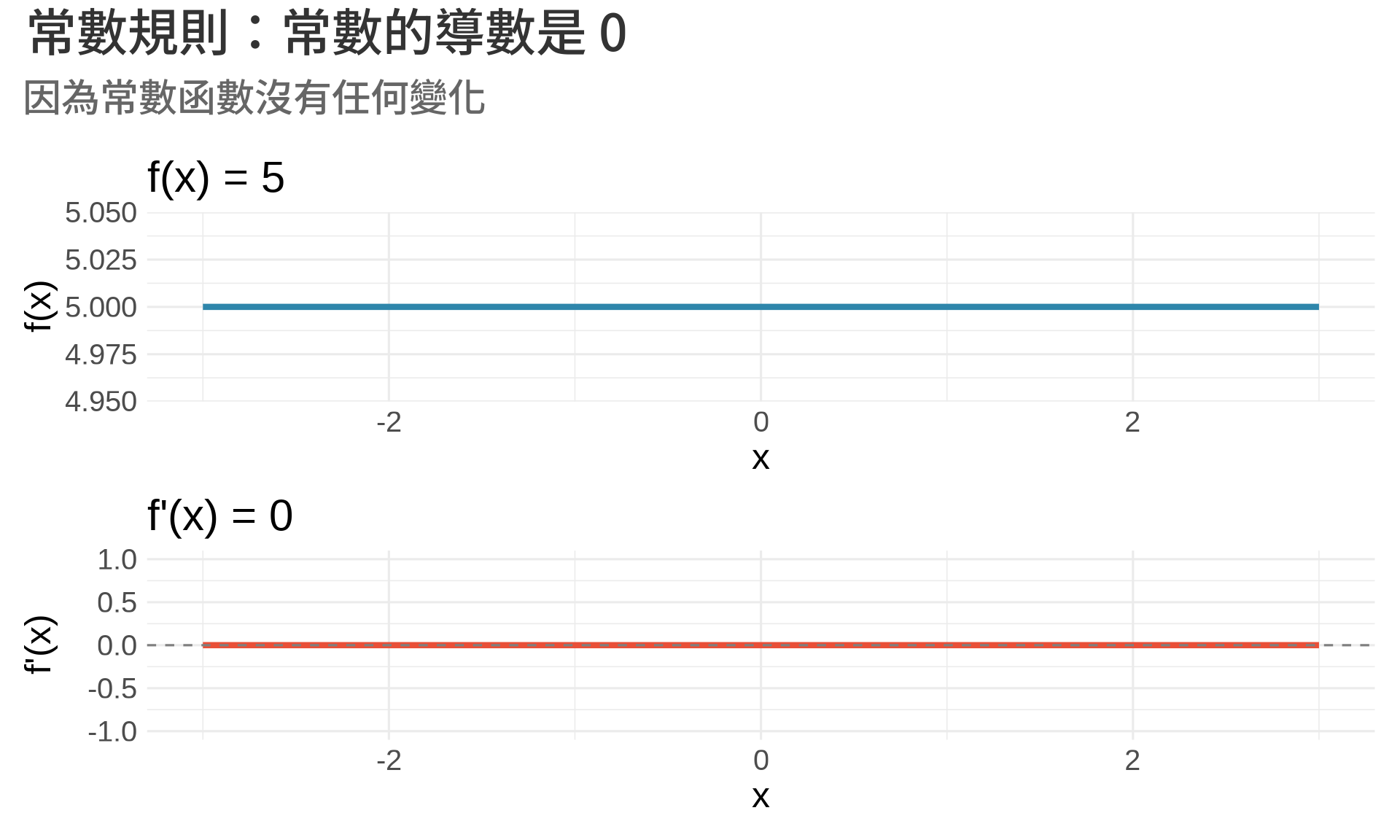
### 1. 常數規則 (Constant Rule)
$$
\frac{d}{dx}(c) = 0
$$
**直觀理解**:常數不會變化,所以變化率是 0。
```{r}
#| label: fig-constant-rule
#| fig-cap: "常數函數的導數恆為 0"
#| warning: false
#| message: false
x <- seq(-3, 3, by = 0.1)
f <- rep(5, length(x))  # f(x) = 5
f_prime <- rep(0, length(x))  # f'(x) = 0

df <- data.frame(x, f, f_prime)

p1 <- ggplot(df, aes(x, f)) +
  geom_line(color = "#2E86AB", linewidth = 1.5) +
  labs(title = "f(x) = 5", y = "f(x)") +
  theme_minimal(base_size = 12)

p2 <- ggplot(df, aes(x, f_prime)) +
  geom_line(color = "#E94F37", linewidth = 1.5) +
  geom_hline(yintercept = 0, linetype = "dashed", color = "gray50") +
  labs(title = "f'(x) = 0", y = "f'(x)") +
  ylim(-1, 1) +
  theme_minimal(base_size = 12)

p1 / p2 +
  plot_annotation(
    title = "常數規則:常數的導數是 0",
    subtitle = "因為常數函數沒有任何變化"
  )
```
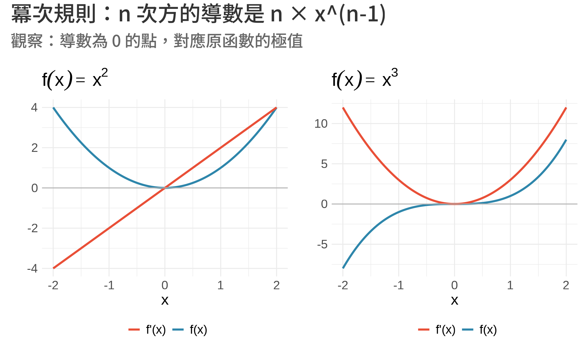
### 2. 冪次規則 (Power Rule)
$$
\frac{d}{dx}(x^n) = nx^{n-1}
$$
這是**最重要**的規則之一!
**範例**:
- $\frac{d}{dx}(x^2) = 2x$
- $\frac{d}{dx}(x^3) = 3x^2$
- $\frac{d}{dx}(x^{10}) = 10x^9$
- $\frac{d}{dx}(\frac{1}{x}) = \frac{d}{dx}(x^{-1}) = -x^{-2} = -\frac{1}{x^2}$
```{r}
#| label: fig-power-rule
#| fig-cap: "冪次規則的視覺化:x² 和 x³ 及其導數"
#| warning: false
#| message: false
x <- seq(-2, 2, by = 0.01)

# x^2 和其導數
f1 <- x^2
f1_prime <- 2*x

# x^3 和其導數
f2 <- x^3
f2_prime <- 3*x^2

df <- data.frame(x, f1, f1_prime, f2, f2_prime)

p1 <- ggplot(df, aes(x)) +
  geom_line(aes(y = f1, color = "f(x)"), linewidth = 1.2) +
  geom_line(aes(y = f1_prime, color = "f'(x)"), linewidth = 1.2) +
  geom_hline(yintercept = 0, color = "gray70") +
  scale_color_manual(values = c("f(x)" = "#2E86AB", "f'(x)" = "#E94F37")) +
  labs(title = expression(f(x) == x^2), y = "", color = "") +
  theme_minimal(base_size = 12) +
  theme(legend.position = "bottom")

p2 <- ggplot(df, aes(x)) +
  geom_line(aes(y = f2, color = "f(x)"), linewidth = 1.2) +
  geom_line(aes(y = f2_prime, color = "f'(x)"), linewidth = 1.2) +
  geom_hline(yintercept = 0, color = "gray70") +
  scale_color_manual(values = c("f(x)" = "#2E86AB", "f'(x)" = "#E94F37")) +
  labs(title = expression(f(x) == x^3), y = "", color = "") +
  theme_minimal(base_size = 12) +
  theme(legend.position = "bottom")

p1 + p2 +
  plot_annotation(
    title = "冪次規則:n 次方的導數是 n × x^(n-1)",
    subtitle = "觀察:導數為 0 的點,對應原函數的極值"
  )
```
**觀察重點**:
- $f(x) = x^2$ 的導數是 $f'(x) = 2x$,在 $x=0$ 處導數為 0(極小值)
- $f(x) = x^3$ 的導數是 $f'(x) = 3x^2$,在 $x=0$ 處導數為 0(反曲點)
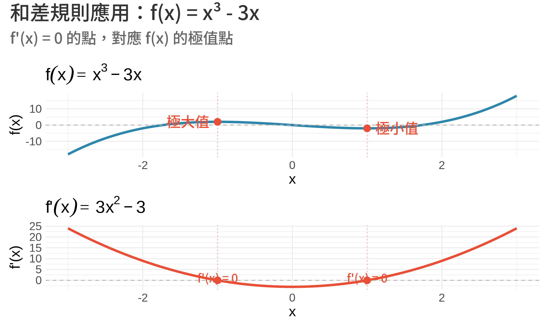
### 3. 和差規則 (Sum/Difference Rule)
$$
\frac{d}{dx}[f(x) + g(x)] = f'(x) + g'(x)
$$
$$
\frac{d}{dx}[f(x) - g(x)] = f'(x) - g'(x)
$$
**範例**:
$$
\frac{d}{dx}(x^3 - 3x) = 3x^2 - 3
$$
這個函數在統計最佳化問題中很常見!
```{r}
#| label: fig-sum-rule
#| fig-cap: "函數與導數的對應關係:極值點在導數為 0 處"
#| warning: false
#| message: false
x <- seq(-3, 3, by = 0.01)

# f(x) = x³ - 3x
f <- x^3 - 3*x
f_prime <- 3*x^2 - 3

df <- data.frame(x, f, f_prime)

# 找極值點:f'(x) = 0 => 3x² - 3 = 0 => x = ±1
extrema_x <- c(-1, 1)
extrema_y <- extrema_x^3 - 3*extrema_x

extrema_df <- data.frame(x = extrema_x, y = extrema_y)

p1 <- ggplot(df, aes(x, f)) +
  geom_line(color = "#2E86AB", linewidth = 1.5) +
  geom_hline(yintercept = 0, color = "gray70", linetype = "dashed") +
  geom_vline(xintercept = extrema_x, color = "#E94F37",
             linetype = "dotted", alpha = 0.5) +
  geom_point(data = extrema_df, aes(x = x, y = y),
             color = "#E94F37", size = 4) +
  annotate("text", x = -1, y = 2, label = "極大值",
           hjust = 1.2, color = "#E94F37") +
  annotate("text", x = 1, y = -2, label = "極小值",
           hjust = -0.2, color = "#E94F37") +
  labs(title = expression(f(x) == x^3 - 3*x), y = "f(x)") +
  theme_minimal(base_size = 12)

extrema_df2 <- data.frame(x = extrema_x, y = c(0, 0))

p2 <- ggplot(df, aes(x, f_prime)) +
  geom_line(color = "#E94F37", linewidth = 1.5) +
  geom_hline(yintercept = 0, color = "gray70", linetype = "dashed") +
  geom_vline(xintercept = extrema_x, color = "#E94F37",
             linetype = "dotted", alpha = 0.5) +
  geom_point(data = extrema_df2, aes(x = x, y = y),
             color = "#E94F37", size = 4) +
  annotate("text", x = -1, y = 1, label = "f'(x) = 0",
           hjust = 0.5, color = "#E94F37", size = 3.5) +
  annotate("text", x = 1, y = 1, label = "f'(x) = 0",
           hjust = 0.5, color = "#E94F37", size = 3.5) +
  labs(title = expression(f*"'"*(x) == 3*x^2 - 3), y = "f'(x)") +
  theme_minimal(base_size = 12)

p1 / p2 +
  plot_annotation(
    title = "和差規則應用:f(x) = x³ - 3x",
    subtitle = "f'(x) = 0 的點,對應 f(x) 的極值點"
  )
```
### 4. 常數倍數規則 (Constant Multiple Rule)
$$
\frac{d}{dx}[c \cdot f(x)] = c \cdot f'(x)
$$
**範例**:
$$
\frac{d}{dx}(5x^2) = 5 \cdot 2x = 10x
$$
### 5. 乘法規則 (Product Rule)
$$
\frac{d}{dx}[f(x) \cdot g(x)] = f'(x) \cdot g(x) + f(x) \cdot g'(x)
$$
**範例**:
$$
\frac{d}{dx}(x^2 \cdot e^x) = 2x \cdot e^x + x^2 \cdot e^x = (2x + x^2)e^x
$$
### 6. 除法規則 (Quotient Rule)
$$
\frac{d}{dx}\left[\frac{f(x)}{g(x)}\right] = \frac{f'(x) \cdot g(x) - f(x) \cdot g'(x)}{[g(x)]^2}
$$
**記憶口訣**:「下導上,減上導下,除以下平方」
**範例**:
$$
\frac{d}{dx}\left(\frac{x}{x^2 + 1}\right) = \frac{1 \cdot (x^2+1) - x \cdot 2x}{(x^2+1)^2} = \frac{1-x^2}{(x^2+1)^2}
$$
## 連鎖律 (Chain Rule) — 最重要的規則!
### 概念
如果 $y = f(g(x))$,也就是「函數套函數」,則:
$$
\frac{dy}{dx} = f'(g(x)) \cdot g'(x)
$$
**白話文**:先對外層函數微分,再乘以內層函數的導數。
**另一種寫法**(Leibniz 記法):
如果 $y = f(u)$ 且 $u = g(x)$,則:
$$
\frac{dy}{dx} = \frac{dy}{du} \cdot \frac{du}{dx}
$$
這個寫法很直觀:就像「約分」一樣!
### 範例 1:$(x^2 + 1)^{10}$
$$
\begin{align}
\text{令 } u &= x^2 + 1, \quad y = u^{10} \\
\frac{dy}{du} &= 10u^9 = 10(x^2+1)^9 \\
\frac{du}{dx} &= 2x \\
\therefore \frac{dy}{dx} &= 10(x^2+1)^9 \cdot 2x = 20x(x^2+1)^9
\end{align}
$$
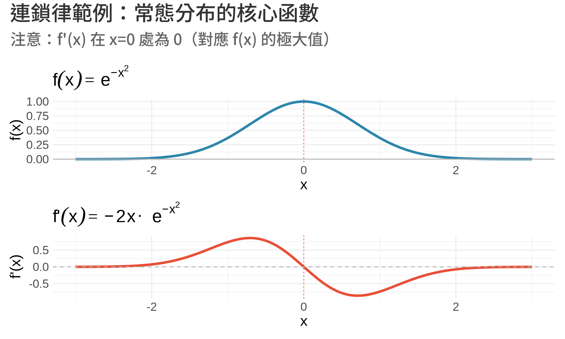
### 範例 2:$e^{x^2}$
$$
\begin{align}
\text{令 } u &= x^2, \quad y = e^u \\
\frac{dy}{du} &= e^u = e^{x^2} \\
\frac{du}{dx} &= 2x \\
\therefore \frac{dy}{dx} &= e^{x^2} \cdot 2x = 2xe^{x^2}
\end{align}
$$
### 視覺化連鎖律
```{r}
#| label: fig-chain-rule
#| fig-cap: "連鎖律視覺化:e^(-x²) 是常態分布的核心"
#| warning: false
#| message: false
x <- seq(-3, 3, by = 0.01)

# f(x) = e^(-x²)
f <- exp(-x^2)
# f'(x) = -2x · e^(-x²)
f_prime <- -2*x * exp(-x^2)

df <- data.frame(x, f, f_prime)

p1 <- ggplot(df, aes(x, f)) +
  geom_line(color = "#2E86AB", linewidth = 1.5) +
  geom_hline(yintercept = 0, color = "gray70") +
  geom_vline(xintercept = 0, color = "#E94F37", linetype = "dotted") +
  labs(title = expression(f(x) == e^{-x^2}), y = "f(x)") +
  theme_minimal(base_size = 12)

p2 <- ggplot(df, aes(x, f_prime)) +
  geom_line(color = "#E94F37", linewidth = 1.5) +
  geom_hline(yintercept = 0, color = "gray70", linetype = "dashed") +
  geom_vline(xintercept = 0, color = "#E94F37", linetype = "dotted") +
  labs(title = expression(f*"'"*(x) == -2*x %.% e^{-x^2}), y = "f'(x)") +
  theme_minimal(base_size = 12)

p1 / p2 +
  plot_annotation(
    title = "連鎖律範例:常態分布的核心函數",
    subtitle = "注意:f'(x) 在 x=0 處為 0(對應 f(x) 的極大值)"
  )
```
**觀察**:
- $f(x) = e^{-x^2}$ 在 $x=0$ 有極大值
- $f'(x) = -2xe^{-x^2}$ 在 $x=0$ 處為 0
- $f'(x)$ 左側為正(上升),右側為負(下降)
## 統計應用
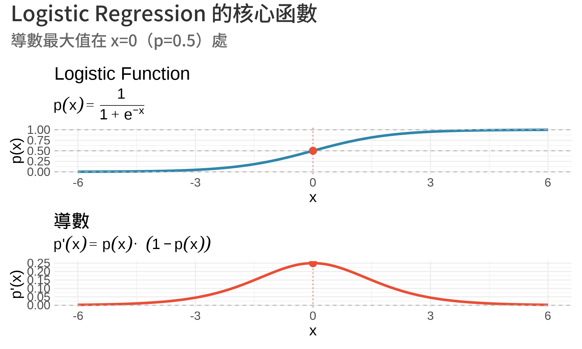
### 1. Logistic Function 的微分
在 logistic regression 中,我們使用 **logistic function**:
$$
p(x) = \frac{1}{1 + e^{-x}} = \frac{e^x}{1 + e^x}
$$
這個函數的導數有個神奇的性質:
$$
p'(x) = p(x) \cdot (1 - p(x))
$$
**推導**(使用除法規則或連鎖律):
$$
\begin{align}
p(x) &= (1 + e^{-x})^{-1} \\
p'(x) &= -(1 + e^{-x})^{-2} \cdot (-e^{-x}) \\
&= \frac{e^{-x}}{(1 + e^{-x})^2} \\
&= \frac{1}{1 + e^{-x}} \cdot \frac{e^{-x}}{1 + e^{-x}} \\
&= p(x) \cdot (1 - p(x))
\end{align}
$$
```{r}
#| label: fig-logistic-derivative
#| fig-cap: "Logistic function 與其導數"
#| warning: false
#| message: false
x <- seq(-6, 6, by = 0.01)

# Logistic function
p <- 1 / (1 + exp(-x))
# 導數
p_prime <- p * (1 - p)

df <- data.frame(x, p, p_prime)

p1 <- ggplot(df, aes(x, p)) +
  geom_line(color = "#2E86AB", linewidth = 1.5) +
  geom_hline(yintercept = c(0, 0.5, 1),
             color = "gray70", linetype = "dashed") +
  geom_vline(xintercept = 0, color = "#E94F37", linetype = "dotted") +
  annotate("point", x = 0, y = 0.5, color = "#E94F37", size = 4) +
  labs(title = "Logistic Function",
       subtitle = expression(p(x) == frac(1, 1 + e^{-x})),
       y = "p(x)") +
  theme_minimal(base_size = 12)

p2 <- ggplot(df, aes(x, p_prime)) +
  geom_line(color = "#E94F37", linewidth = 1.5) +
  geom_hline(yintercept = 0, color = "gray70", linetype = "dashed") +
  geom_vline(xintercept = 0, color = "#E94F37", linetype = "dotted") +
  annotate("point", x = 0, y = 0.25, color = "#E94F37", size = 4) +
  labs(title = "導數",
       subtitle = expression(p*"'"*(x) == p(x) %.% (1 - p(x))),
       y = "p'(x)") +
  theme_minimal(base_size = 12)

p1 / p2 +
  plot_annotation(
    title = "Logistic Regression 的核心函數",
    subtitle = "導數最大值在 x=0(p=0.5)處"
  )
```
**統計意義**:
- Logistic function 將實數映射到 $(0, 1)$,可解釋為機率
- 導數 $p'(x) = p(1-p)$ 在 MLE 推導中非常重要[@casella2002statistical]
- 最大變化率發生在 $p=0.5$ 時
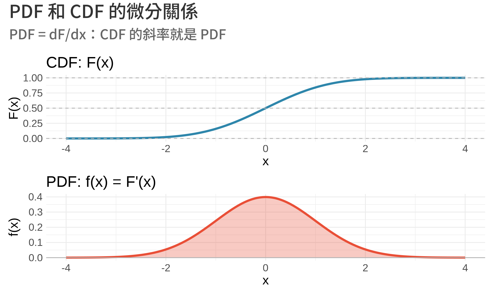
### 2. PDF 和 CDF 的關係
**累積分布函數 (CDF)** 定義為:
$$
F(x) = P(X \le x) = \int_{-\infty}^{x} f(t) dt
$$
根據微積分基本定理,**PDF 是 CDF 的導數**:
$$
f(x) = \frac{d}{dx} F(x) = F'(x)
$$
```{r}
#| label: fig-pdf-cdf
#| fig-cap: "PDF 是 CDF 的導數(標準常態分布)"
#| warning: false
#| message: false
x <- seq(-4, 4, by = 0.01)

# CDF 和 PDF
F_x <- pnorm(x)  # CDF
f_x <- dnorm(x)  # PDF = F'(x)

df <- data.frame(x, F_x, f_x)

p1 <- ggplot(df, aes(x, F_x)) +
  geom_line(color = "#2E86AB", linewidth = 1.5) +
  geom_hline(yintercept = c(0, 0.5, 1),
             color = "gray70", linetype = "dashed") +
  labs(title = "CDF: F(x)", y = "F(x)") +
  theme_minimal(base_size = 12)

p2 <- ggplot(df, aes(x, f_x)) +
  geom_area(fill = "#E94F37", alpha = 0.3) +
  geom_line(color = "#E94F37", linewidth = 1.5) +
  geom_hline(yintercept = 0, color = "gray70") +
  labs(title = "PDF: f(x) = F'(x)", y = "f(x)") +
  theme_minimal(base_size = 12)

p1 / p2 +
  plot_annotation(
    title = "PDF 和 CDF 的微分關係",
    subtitle = "PDF = dF/dx:CDF 的斜率就是 PDF"
  )
```
**觀察**:
- CDF 最陡峭的地方(變化最快),對應 PDF 的峰值
- CDF 平坦的地方(變化緩慢),對應 PDF 接近 0
## 練習題
### 觀念題
1. 用自己的話解釋:為什麼連鎖律叫做 "chain" rule?
::: {.callout-tip collapse="true" title="參考答案"}
因為連鎖律處理的是「函數套函數」的情況,就像一個鏈條(chain)一樣,一環扣一環。外層函數的變化會影響內層函數,內層函數的變化又來自於 x 的變化,這些變化像鏈條一樣連接起來。在數學表達上就是 $\frac{dy}{dx} = \frac{dy}{du} \cdot \frac{du}{dx}$,中間的 du 像「約分」一樣串連起來。
:::
2. 為什麼 PDF 是 CDF 的導數?這在統計上代表什麼意義?
::: {.callout-tip collapse="true" title="參考答案"}
CDF 定義為 $F(x) = \int_{-\infty}^{x} f(t)dt$,根據微積分基本定理,積分的導數就是被積分的函數本身,所以 $f(x) = F'(x)$。統計意義是:PDF 代表「瞬時機率密度」,反映 CDF 在某點的變化率。CDF 變化快的地方(斜率大),PDF 值就大,代表該區域出現的機率密度高。
:::
3. Logistic function 的導數 $p'(x) = p(1-p)$ 在 $p=0$ 和 $p=1$ 時都是 0,這代表什麼?
::: {.callout-tip collapse="true" title="參考答案"}
這代表當機率接近 0 或 1 時,logistic function 的變化率趨近於 0,也就是曲線趨於平坦。從圖形上看,logistic function 是 S 型曲線,兩端漸近於 0 和 1,變化很慢;而在中間 $p=0.5$ 的地方變化最快(導數最大)。這反映了一個重要的統計直覺:當結果幾乎確定時(接近 0% 或 100%),再增加一點 x 值也很難改變機率。
:::
### 計算題
4. 計算下列函數的導數:
a. $f(x) = 3x^4 - 2x^2 + 5$
b. $g(x) = (2x + 1)^5$
c. $h(x) = e^{-2x}$
::: {.callout-tip collapse="true" title="參考答案"}
a. $f'(x) = 12x^3 - 4x$(使用冪次規則和和差規則)
b. $g'(x) = 5(2x+1)^4 \cdot 2 = 10(2x+1)^4$(使用連鎖律)
c. $h'(x) = e^{-2x} \cdot (-2) = -2e^{-2x}$(使用連鎖律,外層是 $e^u$,內層是 $u=-2x$)
:::
5. 使用乘法規則計算:$\frac{d}{dx}(x^2 \ln x)$
::: {.callout-tip collapse="true" title="參考答案"}
使用乘法規則:$\frac{d}{dx}[f \cdot g] = f' \cdot g + f \cdot g'$
令 $f = x^2$,$g = \ln x$,則 $f' = 2x$,$g' = \frac{1}{x}$
因此:$\frac{d}{dx}(x^2 \ln x) = 2x \cdot \ln x + x^2 \cdot \frac{1}{x} = 2x\ln x + x$
:::
6. 使用除法規則計算:$\frac{d}{dx}\left(\frac{x^2}{x+1}\right)$
::: {.callout-tip collapse="true" title="參考答案"}
使用除法規則:$\frac{d}{dx}\left[\frac{f}{g}\right] = \frac{f' \cdot g - f \cdot g'}{g^2}$
令 $f = x^2$,$g = x+1$,則 $f' = 2x$,$g' = 1$
因此:$\frac{d}{dx}\left(\frac{x^2}{x+1}\right) = \frac{2x(x+1) - x^2 \cdot 1}{(x+1)^2} = \frac{2x^2+2x-x^2}{(x+1)^2} = \frac{x^2+2x}{(x+1)^2} = \frac{x(x+2)}{(x+1)^2}$
:::
### R 操作題
7. 繪製 $f(x) = \sin(x^2)$ 和其導數(提示:使用連鎖律)
```{r}
#| eval: false
# 提示
f <- function(x) sin(x^2)
f_prime <- function(x) 2*x * cos(x^2)  # 連鎖律
```
::: {.callout-tip collapse="true" title="參考答案"}
使用連鎖律:外層函數是 $\sin(u)$,內層是 $u=x^2$
$\frac{d}{dx}\sin(x^2) = \cos(x^2) \cdot 2x = 2x\cos(x^2)$
完整程式碼:
```r
library(ggplot2)
library(patchwork)

x <- seq(-3, 3, by = 0.01)
f <- sin(x^2)
f_prime <- 2*x * cos(x^2)

df <- data.frame(x, f, f_prime)

p1 <- ggplot(df, aes(x, f)) +
  geom_line(color = "#2E86AB", linewidth = 1.2) +
  labs(title = expression(f(x) == sin(x^2)), y = "f(x)") +
  theme_minimal()

p2 <- ggplot(df, aes(x, f_prime)) +
  geom_line(color = "#E94F37", linewidth = 1.2) +
  labs(title = expression(f*"'"*(x) == 2*x %.% cos(x^2)), y = "f'(x)") +
  theme_minimal()

p1 / p2
```
:::
8. 驗證 logistic function 的導數公式:計算 $p'(0)$ 的理論值和數值近似值,比較差異。
::: {.callout-tip collapse="true" title="參考答案"}
理論值:$p(0) = \frac{1}{1+e^0} = 0.5$,所以 $p'(0) = p(0)(1-p(0)) = 0.5 \times 0.5 = 0.25$
數值近似(使用導數定義):
```r
# Logistic function
p <- function(x) 1 / (1 + exp(-x))

# 理論導數
p_deriv_theory <- function(x) {
  px <- p(x)
  px * (1 - px)
}

# 數值近似導數
p_deriv_numeric <- function(x, h = 1e-8) {
  (p(x + h) - p(x)) / h
}

# 在 x=0 處比較
theory_val <- p_deriv_theory(0)
numeric_val <- p_deriv_numeric(0)

cat("理論值:", theory_val, "\n")
cat("數值近似值:", numeric_val, "\n")
cat("差異:", abs(theory_val - numeric_val), "\n")
```
結果應該非常接近,差異小於 $10^{-8}$。
:::
## 本章重點整理 {.unnumbered}
:::{.callout-important}
## 核心規則
1. **冪次規則**:$\frac{d}{dx}(x^n) = nx^{n-1}$ — 最基本、最常用
2. **和差規則**:導數可以拆開計算
3. **乘法規則**:$\frac{d}{dx}[f \cdot g] = f' \cdot g + f \cdot g'$
4. **除法規則**:$\frac{d}{dx}\left[\frac{f}{g}\right] = \frac{f' \cdot g - f \cdot g'}{g^2}$
5. **連鎖律**:$\frac{dy}{dx} = \frac{dy}{du} \cdot \frac{du}{dx}$ — **最重要**!
**統計應用**:
- Logistic function 的導數:$p'(x) = p(1-p)$
- PDF = CDF 的導數:$f(x) = F'(x)$
- 極值點滿足 $f'(x) = 0$
**下一章**:我們會專門討論 $e^x$ 和 $\ln x$,了解為什麼統計學特別愛用它們!
:::