# 函數與圖形 {#sec-functions}
```{r}
#| include: false
source(here::here("R/_common.R"))
library(dplyr)
```
## 學習目標 {.unnumbered}
- 理解函數是「輸入對應到輸出」的關係
- 認識常見的函數類型及其圖形特徵
- 能夠用 R 繪製函數圖形
- 連結函數概念與統計模型
## 什麼是函數?
函數是一種「對應關係」:給定一個輸入,就會產生一個確定的輸出。
用數學符號來寫:
$$y = f(x)$$
這表示:當輸入 $x$ 時,函數 $f$ 會產生輸出 $y$。
### 醫學上的函數
在醫學領域,到處都是函數:
- **劑量-反應曲線**:給定藥物劑量(輸入),預測療效(輸出)
- **藥物濃度曲線**:給定時間(輸入),預測血中藥物濃度(輸出)
- **成長曲線**:給定年齡(輸入),預測身高或體重(輸出)
- **風險模型**:給定危險因子(輸入),預測疾病風險(輸出)
## 視覺化理解
### 劑量-反應曲線
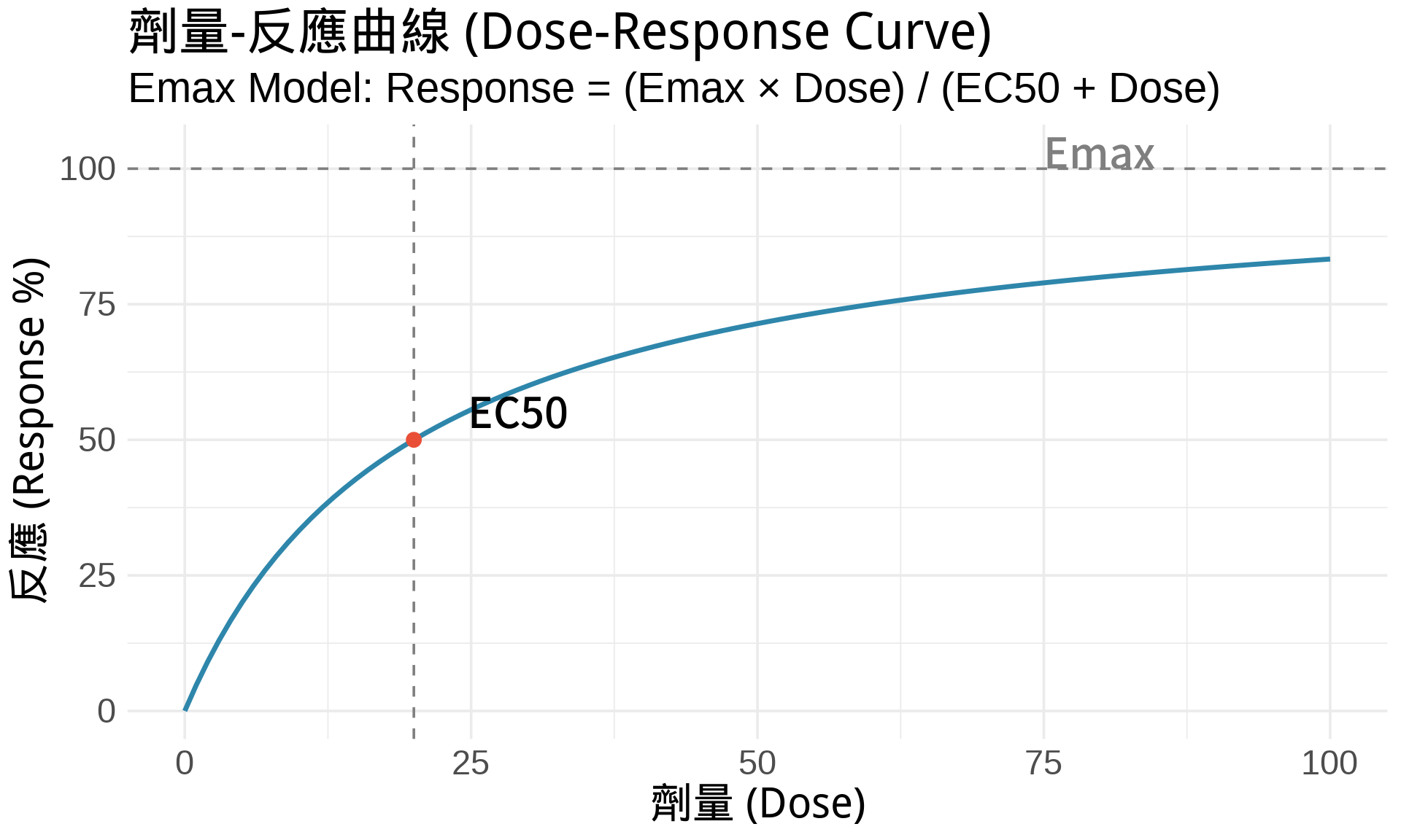
讓我們從一個經典的藥理學例子開始:Emax 模型 [@holford2013pharmacodynamic]。
```{r}
#| fig-cap: "劑量-反應曲線展示了藥物劑量與療效之間的非線性關係"
# 設定參數
dose <- seq(0, 100, by = 1)
emax <- 100  # 最大反應
ec50 <- 20   # 達到 50% 最大反應的劑量

# Emax 模型
response <- (emax * dose) / (ec50 + dose)

# 繪圖
ggplot(data.frame(dose, response), aes(dose, response)) +
  geom_line(color = "#2E86AB", linewidth = 1.2) +
  geom_hline(yintercept = emax, linetype = "dashed", color = "gray50") +
  geom_vline(xintercept = ec50, linetype = "dashed", color = "gray50") +
  annotate("point", x = ec50, y = emax/2, size = 3, color = "#E94F37") +
  annotate("text", x = ec50 + 5, y = emax/2 + 5, label = "EC50", hjust = 0) +
  annotate("text", x = 80, y = emax + 3, label = "Emax", color = "gray50") +
  labs(
    title = "劑量-反應曲線 (Dose-Response Curve)",
    subtitle = "Emax Model: Response = (Emax × Dose) / (EC50 + Dose)",
    x = "劑量 (Dose)",
    y = "反應 (Response %)"
  ) +
  theme_minimal(base_size = 14)
```
這條曲線告訴我們:
- 低劑量時,增加劑量會顯著提升療效
- 高劑量時,療效趨近於飽和(Emax)
- EC50 是達到 50% 最大療效所需的劑量 [@mager2003general]
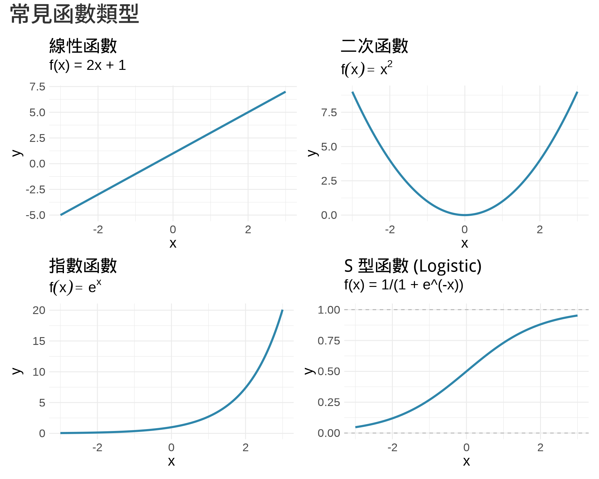
### 常見函數類型
醫學統計中常見的函數類型:
```{r}
#| fig-cap: "四種常見的函數類型"
#| fig-height: 8
x <- seq(-3, 3, by = 0.01)

# 線性函數
p1 <- ggplot(data.frame(x, y = 2*x + 1), aes(x, y)) +
  geom_line(color = "#2E86AB", linewidth = 1.2) +
  labs(title = "線性函數", subtitle = "f(x) = 2x + 1") +
  theme_minimal()

# 二次函數
p2 <- ggplot(data.frame(x, y = x^2), aes(x, y)) +
  geom_line(color = "#2E86AB", linewidth = 1.2) +
  labs(title = "二次函數", subtitle = expression(f(x) == x^2)) +
  theme_minimal()

# 指數函數
p3 <- ggplot(data.frame(x, y = exp(x)), aes(x, y)) +
  geom_line(color = "#2E86AB", linewidth = 1.2) +
  labs(title = "指數函數", subtitle = expression(f(x) == e^x)) +
  theme_minimal()

# S 型函數(Logistic)
p4 <- ggplot(data.frame(x, y = 1/(1 + exp(-x))), aes(x, y)) +
  geom_line(color = "#2E86AB", linewidth = 1.2) +
  geom_hline(yintercept = c(0, 1), linetype = "dashed", color = "gray70") +
  labs(title = "S 型函數 (Logistic)", subtitle = "f(x) = 1/(1 + e^(-x))") +
  theme_minimal()

(p1 | p2) / (p3 | p4) +
  plot_annotation(title = "常見函數類型")
```
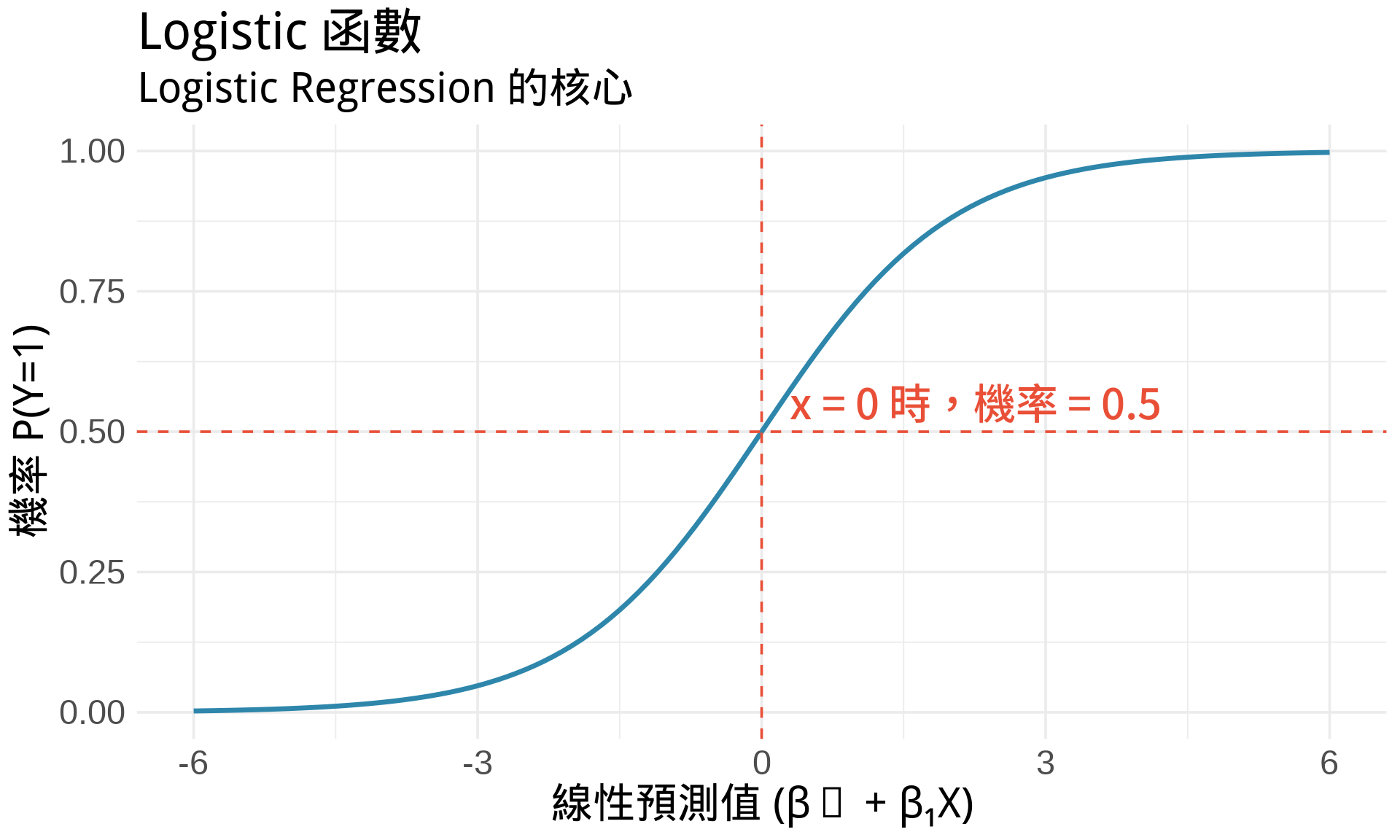
### Logistic 函數的特殊性
在醫學統計中,Logistic 函數特別重要。它將任意實數輸入轉換到 0 和 1 之間,非常適合用來模型化「機率」[@hosmer2013applied]。
```{r}
#| fig-cap: "Logistic 函數將風險因子轉換為機率"
x <- seq(-6, 6, by = 0.1)
prob <- 1 / (1 + exp(-x))

ggplot(data.frame(x, prob), aes(x, prob)) +
  geom_line(color = "#2E86AB", linewidth = 1.2) +
  geom_hline(yintercept = 0.5, linetype = "dashed", color = "#E94F37") +
  geom_vline(xintercept = 0, linetype = "dashed", color = "#E94F37") +
  annotate("text", x = 0.3, y = 0.55, label = "x = 0 時,機率 = 0.5",
           hjust = 0, color = "#E94F37") +
  labs(
    title = "Logistic 函數",
    subtitle = "Logistic Regression 的核心",
    x = "線性預測值 (β₀ + β₁X)",
    y = "機率 P(Y=1)"
  ) +
  scale_y_continuous(breaks = c(0, 0.25, 0.5, 0.75, 1)) +
  theme_minimal(base_size = 14)
```
## 數學定義
### 函數的正式定義
函數 $f: A \to B$ 是一個對應規則,對於集合 $A$ 中的每一個元素 $x$,都恰好對應到集合 $B$ 中的一個元素 $f(x)$。
- $A$ 稱為**定義域** (domain)
- $B$ 稱為**值域** (codomain)
- $f(x)$ 稱為 $x$ 的**函數值** (function value)
### 常見函數的數學形式
| 函數類型 | 數學形式 | 醫學應用 |
|---------|---------|---------|
| 線性 | $f(x) = ax + b$ | 簡單迴歸 |
| 二次 | $f(x) = ax^2 + bx + c$ | U 型關係 |
| 指數 | $f(x) = e^{ax}$ | 細菌生長、藥物代謝 |
| 對數 | $f(x) = \ln(x)$ | 資料轉換 |
| Logistic | $f(x) = \frac{1}{1+e^{-x}}$ | 二元分類 |
## 練習題
### 觀念題
1. 為什麼 Logistic 函數適合用來模型化機率?它的輸出範圍是什麼?
::: {.callout-tip collapse="true" title="參考答案"}
Logistic 函數適合模型化機率,因為無論輸入值為何,其輸出範圍永遠落在 [0, 1] 之間,這正好符合機率的定義。此外,Logistic 函數的 S 型曲線能夠捕捉到「風險因子小時機率接近 0,風險因子大時機率接近 1」的現實情況。
:::
2. 在劑量-反應曲線中,EC50 代表什麼意義?為什麼這個參數在藥理學中很重要?
::: {.callout-tip collapse="true" title="參考答案"}
EC50 代表達到 50% 最大療效(Emax)所需的藥物劑量。這個參數在藥理學中非常重要,因為它反映了藥物的「效價」(potency):EC50 越小,代表藥物越有效,只需較低劑量就能達到顯著療效。EC50 也是不同藥物之間進行效力比較的重要指標。
:::
3. 如果一個函數對同一個輸入可以有多個輸出,它還算是函數嗎?
::: {.callout-tip collapse="true" title="參考答案"}
不算。函數的定義要求每個輸入值必須「恰好」對應到一個輸出值。如果同一個輸入可以產生多個輸出,這種對應關係稱為「關係」(relation),而非函數。例如,$x^2 + y^2 = 1$ 描述的圓形就不是函數,因為給定一個 $x$ 值可能對應到兩個 $y$ 值。
:::
### 計算題
1. 若 $f(x) = x^2 - 3x + 2$,計算 $f(0)$、$f(1)$、$f(2)$。
::: {.callout-tip collapse="true" title="參考答案"}
代入各個 $x$ 值計算:
- $f(0) = 0^2 - 3(0) + 2 = 2$
- $f(1) = 1^2 - 3(1) + 2 = 0$
- $f(2) = 2^2 - 3(2) + 2 = 0$
:::
2. 若 Emax = 100,EC50 = 25,計算劑量為 50 時的反應值。
::: {.callout-tip collapse="true" title="參考答案"}
使用 Emax 模型公式:Response = (Emax × Dose) / (EC50 + Dose)
Response = (100 × 50) / (25 + 50) = 5000 / 75 ≈ 66.7
當劑量為 50(恰好是 EC50 的兩倍)時,反應值約為 66.7%,已經超過最大療效的一半。
:::
### R 操作題
1. 修改劑量-反應曲線的程式碼,將 EC50 改為 10,觀察曲線如何變化。
```{r}
#| eval: false
# 修改這段程式碼
dose <- seq(0, 100, by = 1)
emax <- 100
ec50 <- 10  # 改為 10

response <- (emax * dose) / (ec50 + dose)

ggplot(data.frame(dose, response), aes(dose, response)) +
  geom_line(color = "#2E86AB", linewidth = 1.2) +
  theme_minimal()
```
::: {.callout-tip collapse="true" title="參考答案"}
當 EC50 從 20 降為 10 時,曲線會更快達到飽和:在較低劑量時就能達到接近最大療效。曲線的「轉折點」會向左移動,這表示藥物效價提高了。在實際藥理學中,EC50 較小的藥物被認為效力更強。
:::
2. 繪製對數函數 $f(x) = \ln(x)$ 在 $x \in (0, 10]$ 的圖形。
::: {.callout-tip collapse="true" title="參考答案"}
使用 `stat_function()` 或直接計算即可:
```r
x <- seq(0.01, 10, by = 0.01)
y <- log(x)
ggplot(data.frame(x, y), aes(x, y)) +
  geom_line(color = "#2E86AB", linewidth = 1.2) +
  labs(title = "對數函數", x = "x", y = "ln(x)") +
  theme_minimal()
```
你會觀察到對數函數在 $x$ 接近 0 時趨向負無窮,當 $x = 1$ 時等於 0,之後緩慢增長。
:::
## 統計應用
函數的概念是所有統計模型的基礎 [@mould2012basic]:
| 統計方法 | 使用的函數形式 | 章節連結 |
|---------|--------------|---------|
| 線性迴歸 | $E[Y] = \beta_0 + \beta_1 X$ | @sec-regression |
| Logistic 迴歸 | $\log\frac{p}{1-p} = \beta_0 + \beta_1 X$ | @sec-regression |
| 存活分析 | $S(t) = e^{-\lambda t}$ | @sec-survival |
| 貝氏統計 | 先驗 × Likelihood ∝ 後驗 | @sec-bayesian |
在接下來的章節中,我們會學習如何分析這些函數的「變化率」(微分)和「累積效應」(積分)。
## 本章重點整理 {.unnumbered}
- 函數是「輸入對應到輸出」的確定關係
- 常見函數類型:線性、二次、指數、對數、Logistic
- Logistic 函數在醫學統計中特別重要,因為它將實數映射到 [0, 1] 區間
- 所有統計模型本質上都是在描述變數之間的函數關係
- 用 `ggplot2` 繪製函數圖形是理解函數行為的好方法