7 Time-Varying Exposures

When treatment or exposure status changes during follow-up, standard Cox regression with a baseline-only covariate introduces immortal time bias. This module implements landmark analysis and time-dependent Cox models to handle this correctly.

7.1 Immortal Time Bias

A Common Mistake

If treatment is received at some point after baseline, the time between baseline and treatment receipt is “immortal” — the patient must survive to receive treatment. Coding treatment as a fixed baseline variable credits this survival time to the treatment group, biasing the hazard ratio downward¹.

flowchart LR
    A[Baseline] -->|Immortal time| B[Treatment received]
    B -->|Follow-up| C[Event or censoring]
    A -->|Naive analysis credits<br/>all time to treatment| C

7.2 Script Pipeline

Script	Purpose
`01_landmark_analysis.R`	Landmark analysis at fixed time points
`02_tdc_data_prep.R`	Prepare counting-process data with `tmerge`
`03_tdc_cox.R`	Time-dependent Cox model
`04_immortal_time_check.R`	Compare naive vs corrected estimates
`05_visualization.R`	Forest plot of naive vs corrected HR

7.3 Landmark Analysis

Landmark analysis restricts the cohort to patients alive and event-free at a fixed landmark time, classifying treatment status as of that moment:

landmark_time <- 90  # days

df_landmark <- df |>
  filter(time > landmark_time) |>
  mutate(
    treatment = ifelse(treatment_date <= landmark_time, 1, 0),
    time_from_landmark = time - landmark_time
  )

coxph(Surv(time_from_landmark, status) ~ treatment + age, data = df_landmark)

Choosing the Landmark

The landmark time should be clinically motivated (e.g., 90 days post-diagnosis for transplant studies). Sensitivity analyses at multiple landmarks strengthen the finding.

7.4 Time-Dependent Cox with tmerge

For a more flexible approach, tmerge creates counting-process intervals that update exposure status at the exact time of change:

library(survival)

df_td <- tmerge(df, df, id = id, tstop = time) |>
  tmerge(treatment_df, id = id, trt = tdc(treatment_date))

td_fit <- coxph(Surv(tstart, tstop, status) ~ trt + age, data = df_td)
summary(td_fit)

7.5 Naive vs Corrected Comparison

Script 04_immortal_time_check.R fits both the naive (fixed baseline) and corrected (time-dependent) models side by side:

Naive HR:     0.62 (0.48-0.80)   # biased downward
Corrected HR: 0.85 (0.65-1.11)   # unbiased

Always Report Both

Showing the naive and corrected estimates together makes the magnitude of immortal time bias explicit, which strengthens the manuscript’s methodological rigour.

7.6 Running the Module

make analyze-time-varying PROJECT=my-study

7.7 Demo: Immortal Time Bias (Scenario 5)

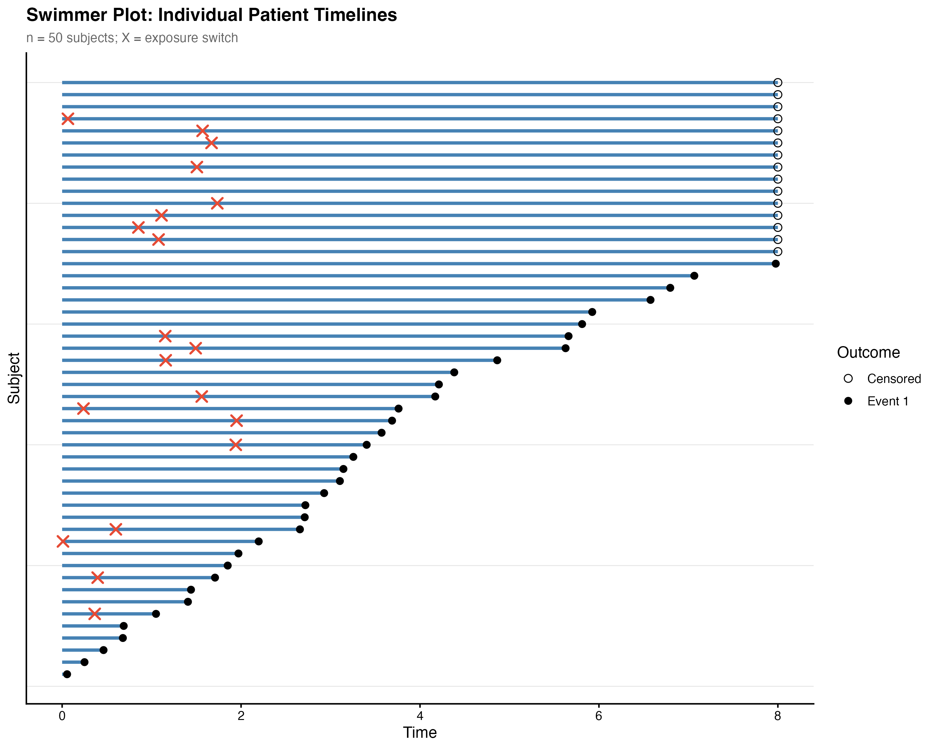
N=800, treatment switch at random time for 33.6% of patients (269/800). True HR = 0.80.

7.7.1 The Bias Revealed

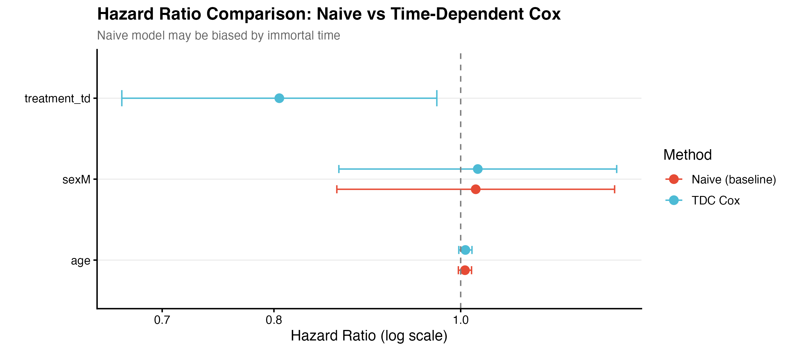
The naive analysis assigned treatment as a fixed baseline variable. Because all patients start untreated and only some switch later, the naive model cannot estimate a treatment HR (the baseline treatment coefficient is NA). The time-dependent Cox model correctly handles the switching and recovers HR = 0.805 (95% CI: 0.667–0.972, p = 0.024), close to the true value of 0.80.

Table 7.1: Naive vs time-dependent Cox comparison

Method	Treatment HR	95% CI	p-value
Naive (baseline)	NA	–	–
Time-dependent Cox	0.805	0.667–0.972	0.024

Warning

The naive analysis cannot estimate the treatment HR because all patients start untreated. The time-dependent Cox correctly identifies HR = 0.805 (p = 0.024).

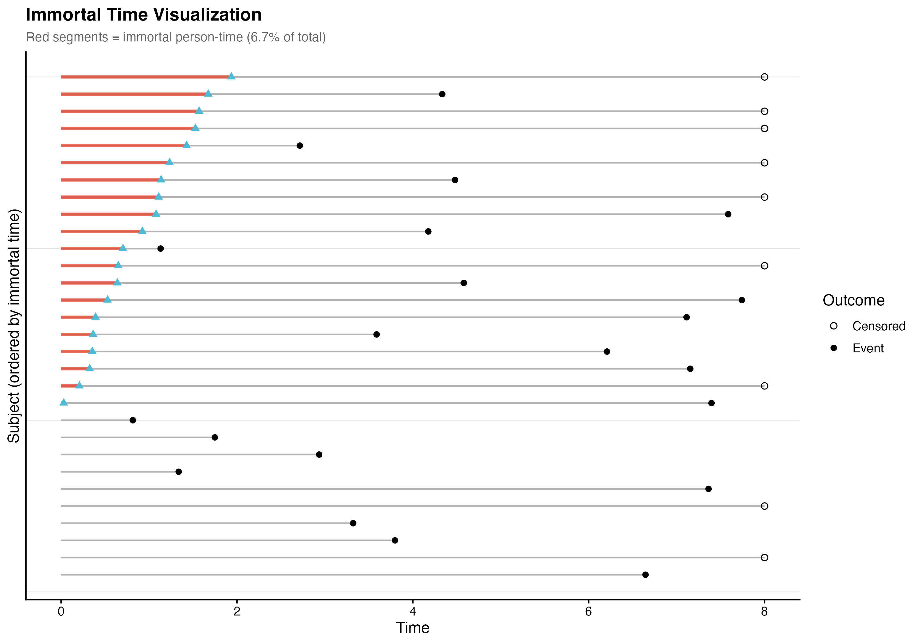
Figure 7.1: Comparison of naive vs time-dependent Cox HRs

7.7.2 Immortal Time Quantification

Of the total 3736 person-time units of follow-up, 249.5 units (6.68%) constituted immortal person-time — time during which switchers were misclassified as treated but had not yet received treatment. The mean immortal time per switcher was 0.93 time units (median 0.83).

Table 7.2: Immortal time summary

Metric	Value
Total person-time	3736.0
Total immortal time	249.5
% immortal	6.68%
Mean immortal time per switcher	0.93
Median immortal time per switcher	0.83

Figure 7.2: Visualization of immortal person-time

7.7.3 Swimmer Plot

Figure 7.3: Individual patient timelines showing treatment switches

7.7.4 Landmark Analysis

Suissa S. Immortal time bias in pharmacoepidemiology. American Journal of Epidemiology. 2008;167(4):492-499.