6 Recurrent Events & Multi-State Models

When subjects experience the same event more than once (recurrent hospitalisations, infections, relapses), standard Cox regression is invalid because it assumes one event per subject. This module provides three recurrent-event frameworks and a multi-state modelling approach.

6.1 Recurrent Event Models

Model	Assumption	Strengths	Limitations
Andersen-Gill (AG)	Events are independent	Simple extension of Cox	Ignores event ordering
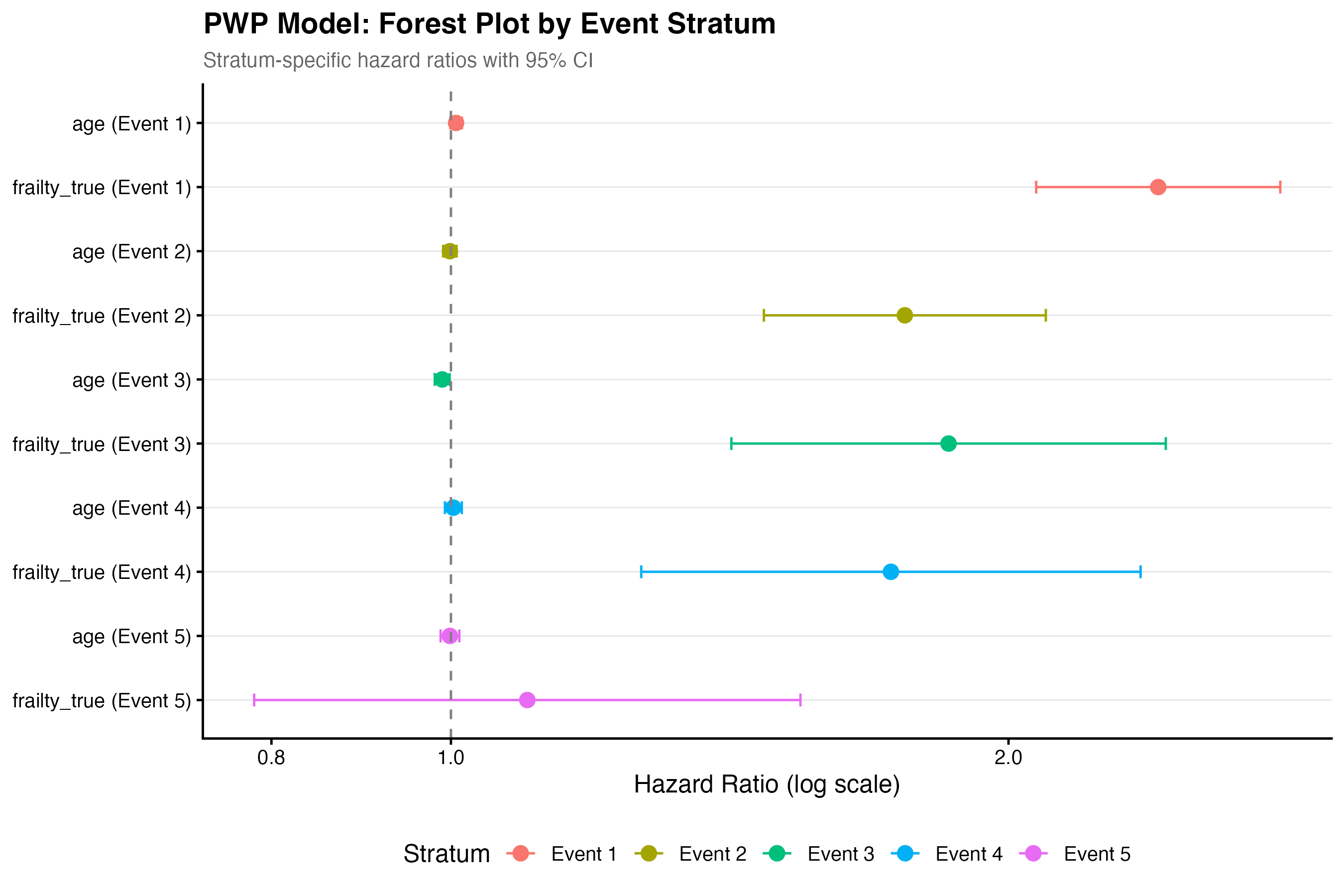
Prentice-Williams-Peterson (PWP)	Event-order matters	Stratifies by event number	Sparse data in later strata
Wei-Lin-Weissfeld (WLW)	Marginal model	Robust to dependence structure	Less efficient
Frailty	Subject-level random effect	Models heterogeneity	Distributional assumption

Choosing a Model

AG is the default for recurrent events. Use PWP when event ordering is clinically meaningful (e.g., 1st vs 2nd relapse differs). Use frailty when between-subject heterogeneity is the scientific question¹.

6.2 Script Pipeline

Script	Purpose
`01_recurrent_descriptive.R`	Event frequency tables, gap-time summaries
`02_ag_model.R`	Andersen-Gill counting process model
`03_pwp_model.R`	Prentice-Williams-Peterson gap-time model
`04_wlw_model.R`	Wei-Lin-Weissfeld marginal model
`05_frailty_recurrent.R`	Gamma frailty for recurrent events
`06_multistate_setup.R`	Define states and transitions with `mstate`
`07_multistate_models.R`	Fit transition-specific Cox models
`08_multistate_plots.R`	State occupation probabilities

6.3 Andersen-Gill Example

library(survival)

ag_fit <- coxph(
  Surv(tstart, tstop, status) ~ group + age + cluster(id),
  data = df_counting
)
summary(ag_fit)

The cluster(id) term provides robust sandwich standard errors to account for within-subject correlation.

6.4 Multi-State Models

For complex disease trajectories (e.g., healthy -> diseased -> dead, with possible recovery), the multi-state module uses the mstate package:

library(mstate)

tmat <- transMat(x = list(c(2, 3), c(3), c()),
                 names = c("Healthy", "Disease", "Dead"))
msdata <- msprep(data = df, trans = tmat,
                 time = c(NA, "t_disease", "t_death"),
                 status = c(NA, "s_disease", "s_death"))

Visualisation

Script 08_multistate_plots.R generates stacked state-occupation probability plots — useful for showing how the proportion of patients in each state evolves over time.

6.5 Running the Module

make analyze-recurrent PROJECT=my-study

6.6 Demo: Recurrent Events (Scenario 3)

N=400 patients with up to 5 recurrent infections and terminal death event. Gamma frailty (variance=0.5).

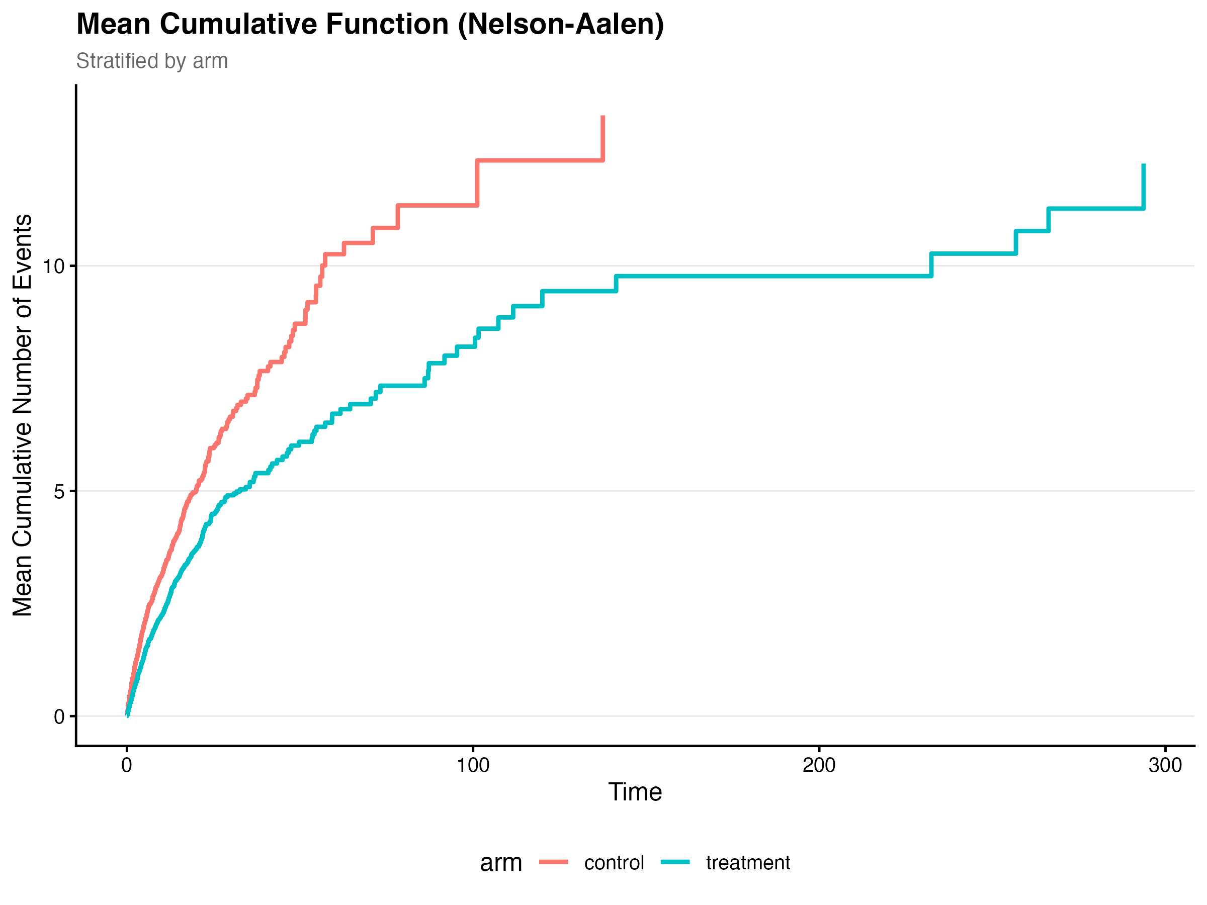
6.6.1 Mean Cumulative Function

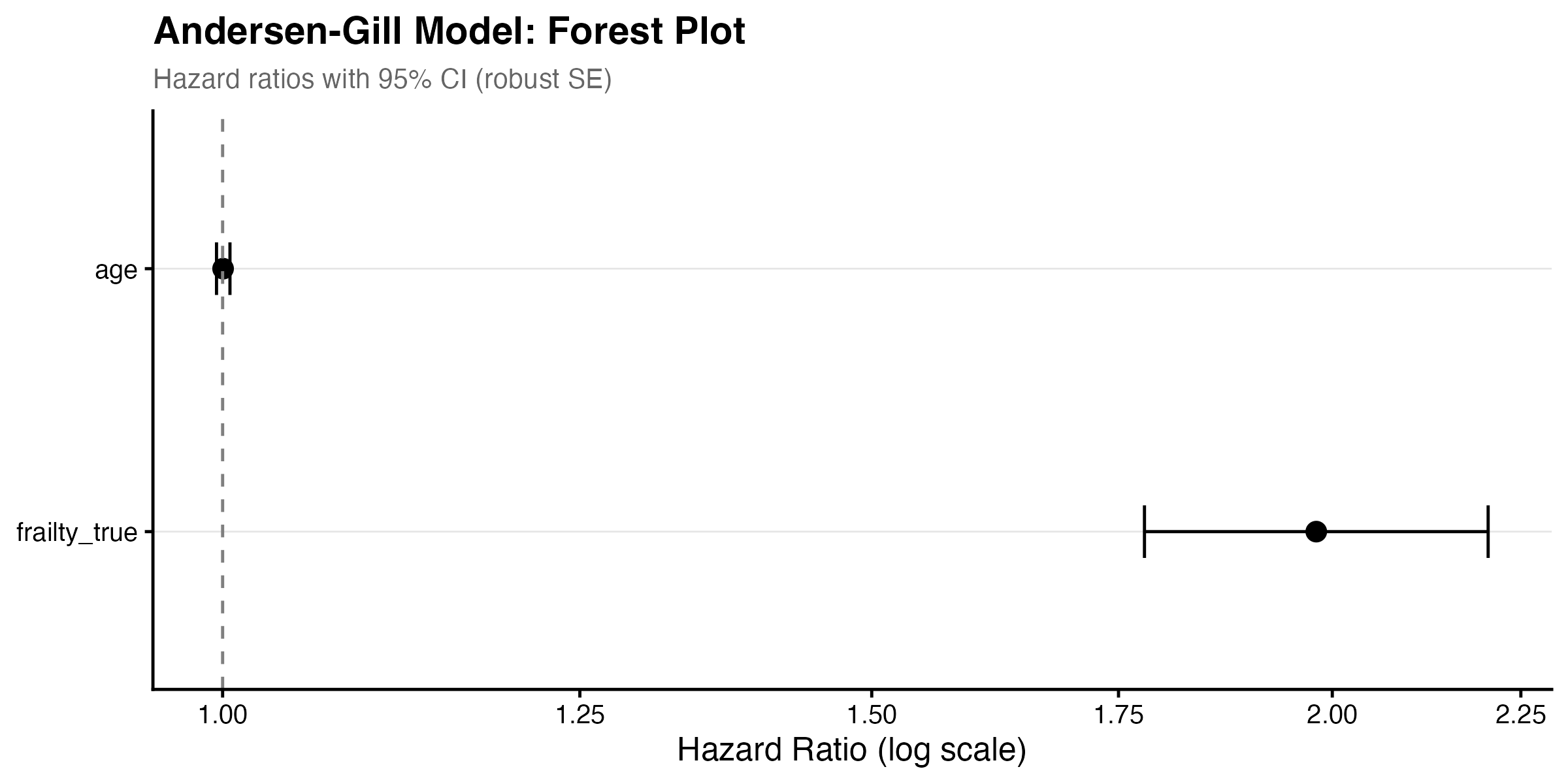
Figure 6.1: Nelson-Aalen MCF by treatment arm

6.6.2 Model Comparison

The Andersen-Gill model estimated a frailty HR of 1.98 (95% CI: 1.78–2.20, p < 0.001), confirming that higher underlying frailty strongly predicts recurrent infections. Age was non-significant (HR = 1.00, p = 0.87). Event rates differed substantially between arms: control 0.254 events/person-time (651 events across 204 subjects) versus treatment 0.148 events/person-time (551 events across 196 subjects).

Table 6.1: Andersen-Gill model results

Variable	HR	95% CI	p-value
Frailty (true)	1.98	1.78–2.20	< 0.001
Age	1.00	1.00–1.00	0.870

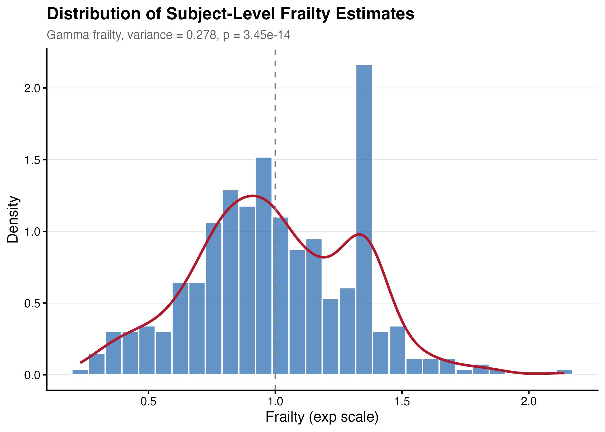
Figure 6.2: Andersen-Gill model forest plot

6.6.3 Frailty Estimation

The gamma frailty model estimated a frailty variance of 0.278, which is lower than the true simulated variance of 0.50. This attenuation is expected — frailty variance is notoriously difficult to estimate and tends to be biased downward in finite samples.

Figure 6.4: Estimated frailty distribution

6.6.4 Terminal Event

Figure 6.5: KM curve for terminal event (death)

Andersen PK, Gill RD. Cox’s regression model for counting processes: A large sample study. The Annals of Statistics. 1982;10(4):1100-1120.