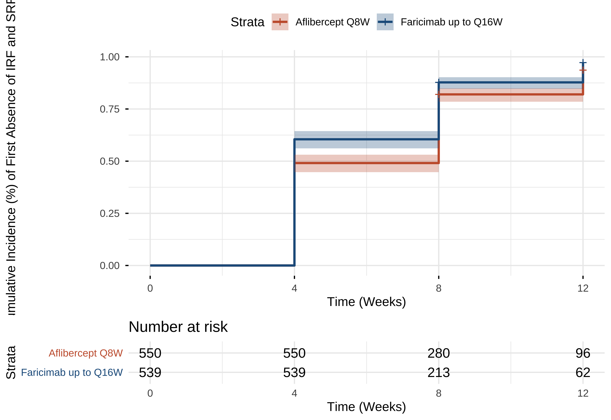
# Part 6(Bonus):Figure 3 — Time to first absence of fluid ```{r} #| label: setup-part6 #| include: false source ("_common.R" )library (readr)library (dplyr)library (tidyr)library (survival)library (survminer)library (broom)<- read_csv ("data/faricimab_baseline.csv" , show_col_types = FALSE )<- read_csv ("data/faricimab_followup.csv" , show_col_types = FALSE )``` - **Kaplan–Meier 教學**:Jager 2008 *Kidney Int*[ @jager2008km ] 、Rich 2010 practical guide[ @rich2010km ] - **Survival in clinical trials**:Fleming & Lin 2000 *Biometrics*[ @fleming2000survival ] - **Proportional hazards 假設檢定(Schoenfeld residuals 等)**:Hess 1995 *Stat Med*[ @hess1995phgraphic ] - **非比例 hazards(NPH)的處理**:Gregson 2019 *JACC*[ @gregson2019nph ] > AI 對 Cox 模型的 PH 假設、log-rank 與 weighted log-rank 的差別、以及 cumulative incidence 與 KM survival 的視覺翻轉**常常給錯**。本章把 Cheung 2025 paper 的 KM cumulative incidence 風格 reproduce,PH assumption 用 `cox.zph()` 檢查(範例見 `appendix.qmd` )。 ::: > 我有 R data frame `baseline` 與 `followup` 。請給我 R code: > > 1. 從 baseline 篩出「有 IRF 或 SRF」的病人(樣本量 ≈ 1170) > 2. 把 followup 加上 baseline 的 arm 與 baseline IRF/SRF > 3. 對每個病人找出第一個 IRF=0 且 SRF=0 的 visit (week 4/8/12),作為 time-to-event;沒事件則 censored at last visit > 4. 用 `survival::survfit(Surv(time, event) ~ arm)` 跑 KM > 5. 用 `survminer::ggsurvplot()` 畫圖(cumulative incidence,亦即 1-KM) > 6. 用 `survival::coxph()` 拿 hazard ratio + 95% CI + log-rank p ::: ## 任務 25:什麼是 time-to-event analysis? > 用「給沒學過統計的眼科醫師聽得懂」的方式 100 字內解釋: > 1. 什麼是 time-to-event? > 2. 什麼是 censoring? > 3. 為什麼不能用 mean / proportion 比較「事件發生時間」? > 4. 什麼是 hazard ratio? - **事件**:第一次 IRF + SRF 都消失(在 OCT 上看不到 fluid)- **censoring**:到追蹤結束都沒事件的病人;不能直接刪、會偏 bias[ @jager2008km ] - **Kaplan–Meier**:把「直到 t 時間還沒事件」的比例畫出來,會階梯狀下降[ @rich2010km; @fleming2000survival ] - **Hazard ratio = 1.47**:faricimab 比 aflibercept 的「事件發生 instantaneous rate」高 47%[ @hess1995phgraphic ] 。`cox.zph()` )。[ @gregson2019nph ] 。## 任務 26:建立 time-to-event dataset ```{r} #| label: build-tte # ── 前置(可單獨執行):套件 + 資料 ── library (readr); library (dplyr); library (tidyr)library (survival); library (survminer); library (broom)<- read_csv ("data/faricimab_baseline.csv" , show_col_types = FALSE )<- read_csv ("data/faricimab_followup.csv" , show_col_types = FALSE )# Cohort:baseline 有 IRF 或 SRF 的病人(per paper:n_fari=581, n_afli=591) <- baseline |> filter (irf_baseline == 1 | srf_baseline == 1 ) |> select (patient_id, arm)cat ("Eligible n:" , nrow (elig), " \n " )cat (" faricimab :" , sum (elig$ arm == "faricimab" ), " \n " )cat (" aflibercept:" , sum (elig$ arm == "aflibercept" ), " \n " )# 對每個病人找第一個 IRF=0 & SRF=0 的 visit <- followup |> filter (patient_id %in% elig$ patient_id) |> mutate (both_absent = (irf == 0 & srf == 0 )) |> group_by (patient_id) |> arrange (week) |> summarise (first_event_week = suppressWarnings (min (week[! is.na (both_absent) & both_absent])last_visit_week = suppressWarnings (max (week[! is.na (both_absent)]).groups = "drop" |> mutate (event = is.finite (first_event_week),time = if_else (event, first_event_week, last_visit_week),time = if_else (is.infinite (time), 12 , time) # default censor at end |> left_join (elig, by = "patient_id" ) |> mutate (arm = factor (arm, levels = c ("aflibercept" ,"faricimab" )))head (tte)``` ## 任務 27:畫 KM curve(cumulative incidence 形式) > 用 `survminer::ggsurvplot()` 畫 cumulative incidence(fun="event"),by arm。x 從 0 到 12 週。 > faricimab 深藍 #1F5C8B、aflibercept 赭橙 #C75D38。 ### 參考程式碼 ```{r} #| label: km-fit # ── 前置(可單獨執行):套件 + 資料 ── library (readr); library (dplyr); library (tidyr)library (survival); library (survminer); library (broom)<- read_csv ("data/faricimab_baseline.csv" , show_col_types = FALSE )<- read_csv ("data/faricimab_followup.csv" , show_col_types = FALSE )# ⚠️ 沿用前面任務的物件:tte(請先跑完任務26,本段不重算) <- survfit (Surv (time, event) ~ arm, data = tte)``` ```{r} #| label: fig3-km #| fig-cap: "Figure 3. Reproduced — Time to first absence of IRF and SRF in patients with IRF or SRF at baseline." #| fig-width: 8 #| fig-height: 5.5 <- ggsurvplot (data = tte,fun = "event" , # cumulative incidence (1 - S(t)) conf.int = TRUE ,risk.table = TRUE ,risk.table.height = 0.25 ,palette = c ("#C75D38" , "#1F5C8B" ),legend.labs = c ("Aflibercept Q8W" , "Faricimab up to Q16W" ),xlab = "Time (Weeks)" ,ylab = "Cumulative Incidence (%) of First Absence of IRF and SRF" ,break.time.by = 4 ,ggtheme = theme_minimal (base_size = 12 ) + theme (legend.position = "bottom" )``` ## 任務 28:Cox 回歸 — Hazard ratio > 用 `survival::coxph(Surv(time, event) ~ arm + study + bcva_strat + lld_strat + region, data = tte)` 算 stratified Cox model。回傳 hazard ratio + 95% CI + log-rank p。 ### 參考程式碼 ```{r} #| label: cox-model # ── 前置(可單獨執行):套件 + 資料 ── library (readr); library (dplyr); library (tidyr)library (survival); library (survminer); library (broom)<- read_csv ("data/faricimab_baseline.csv" , show_col_types = FALSE )<- read_csv ("data/faricimab_followup.csv" , show_col_types = FALSE )# ⚠️ 沿用前面任務的物件:tte(請先跑完任務26,本段不重算) <- tte |> left_join (|> select (patient_id, study, bcva_strat, lld_strat, region),by = "patient_id" |> mutate (study = factor (study),bcva_strat = factor (bcva_strat),lld_strat = factor (lld_strat),region = factor (region)<- coxph (Surv (time, event) ~ arm + study + bcva_strat + lld_strat + region,data = tte_fullsummary (m_cox)``` ```{r} #| label: cox-tidy tidy (m_cox, exponentiate = TRUE , conf.int = TRUE ) |> filter (grepl ("^arm" , term)) |> select (term, hazard_ratio = estimate, lower = conf.low,upper = conf.high, p.value)``` ## 整合:你下課帶回家的東西 | 檔案 | 內容 | |---|---| | `_book/` | 渲染好的整本 HTML 教材,可瀏覽 | | `data/faricimab_baseline.csv` 等 | 模擬資料 | | `scripts/01_table1.R` 等 | 5 支獨立可跑的 R 腳本 | | 你自己跑出的圖 | Table 1、Fig 1A/B、Fig 2 三 panel、Fig 3 KM | | `data/data_dictionary.md` | 院內 csv schema | | `appendix.qmd` | 院內換資料時的常見錯誤 | 1. Time-to-event 多了一個維度:**「事件發生有多快」**2. KM 是 non-parametric、Cox 是 semi-parametric;前者畫圖、後者算 HR3. Cumulative incidence (1-KM) 是 paper 慣用的展示方式4. 三個 method(MMRM、CMH、Cox)放一起就是一篇 phase 3 nAMD paper 的骨架