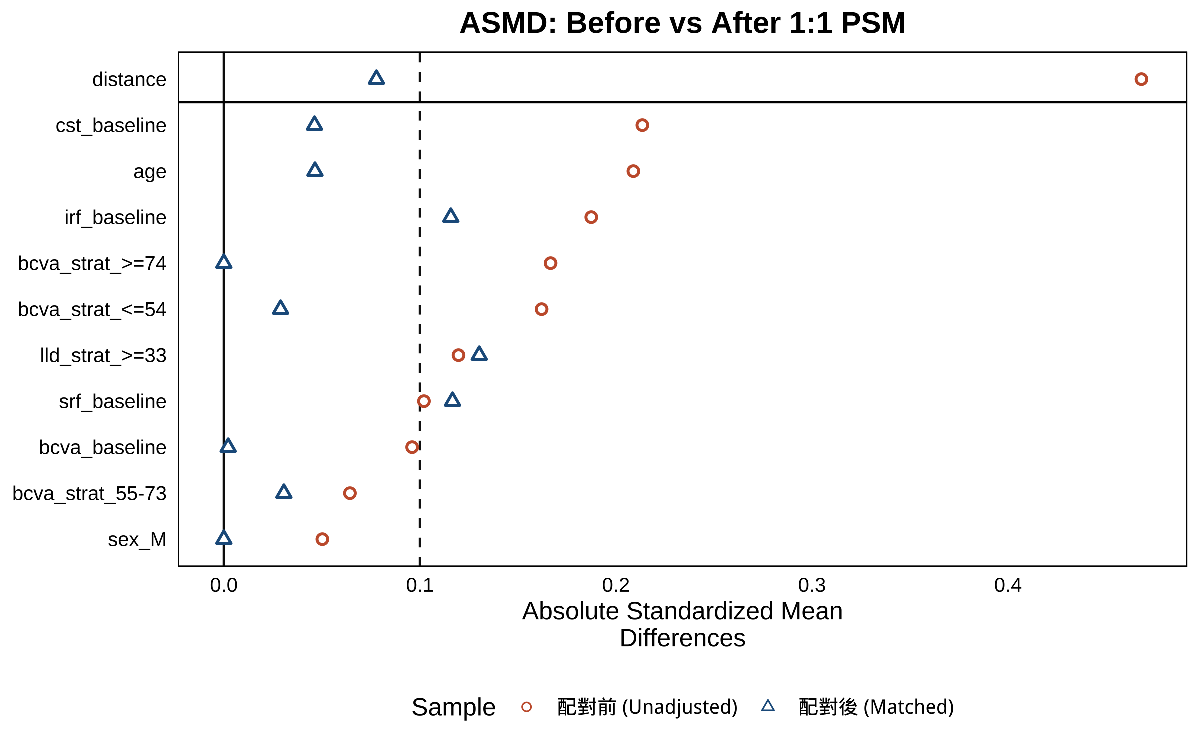
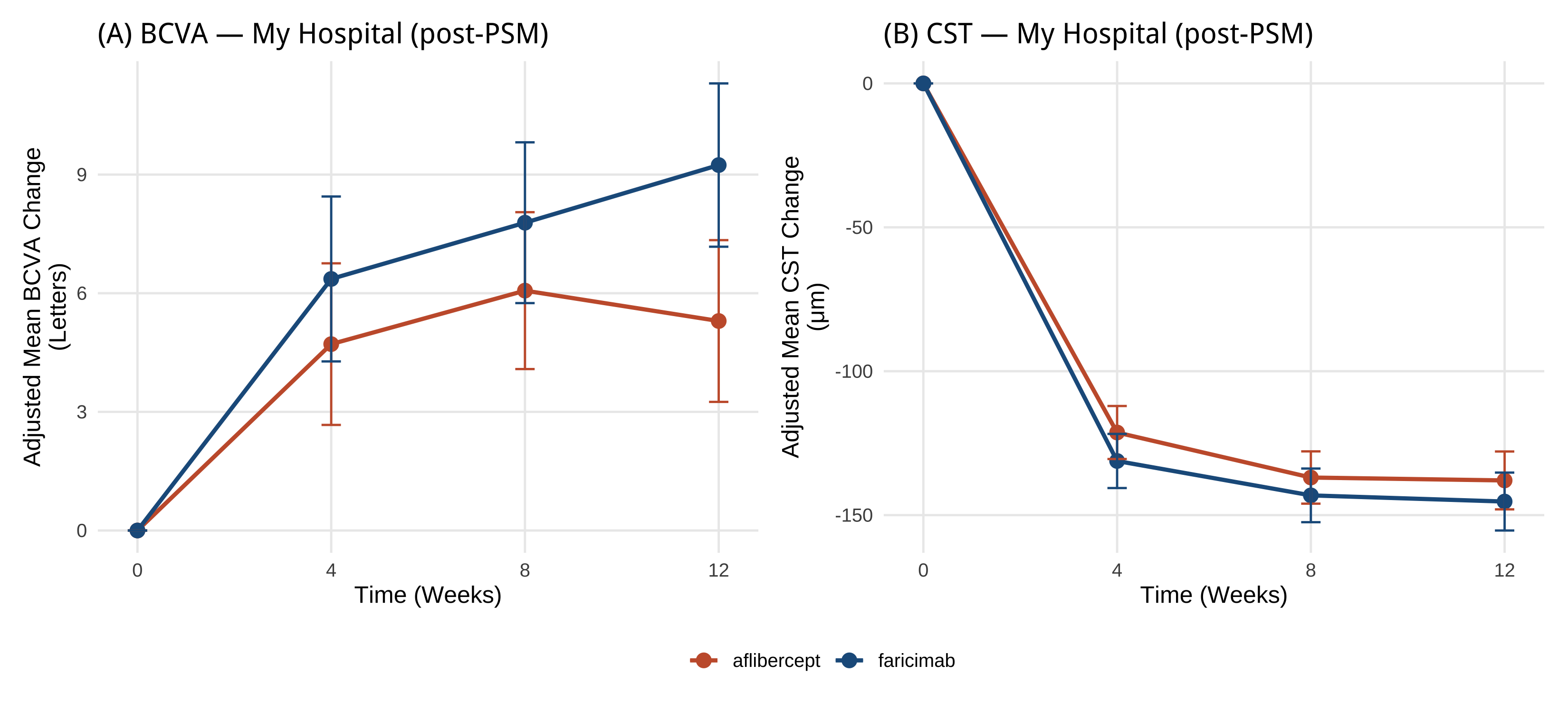
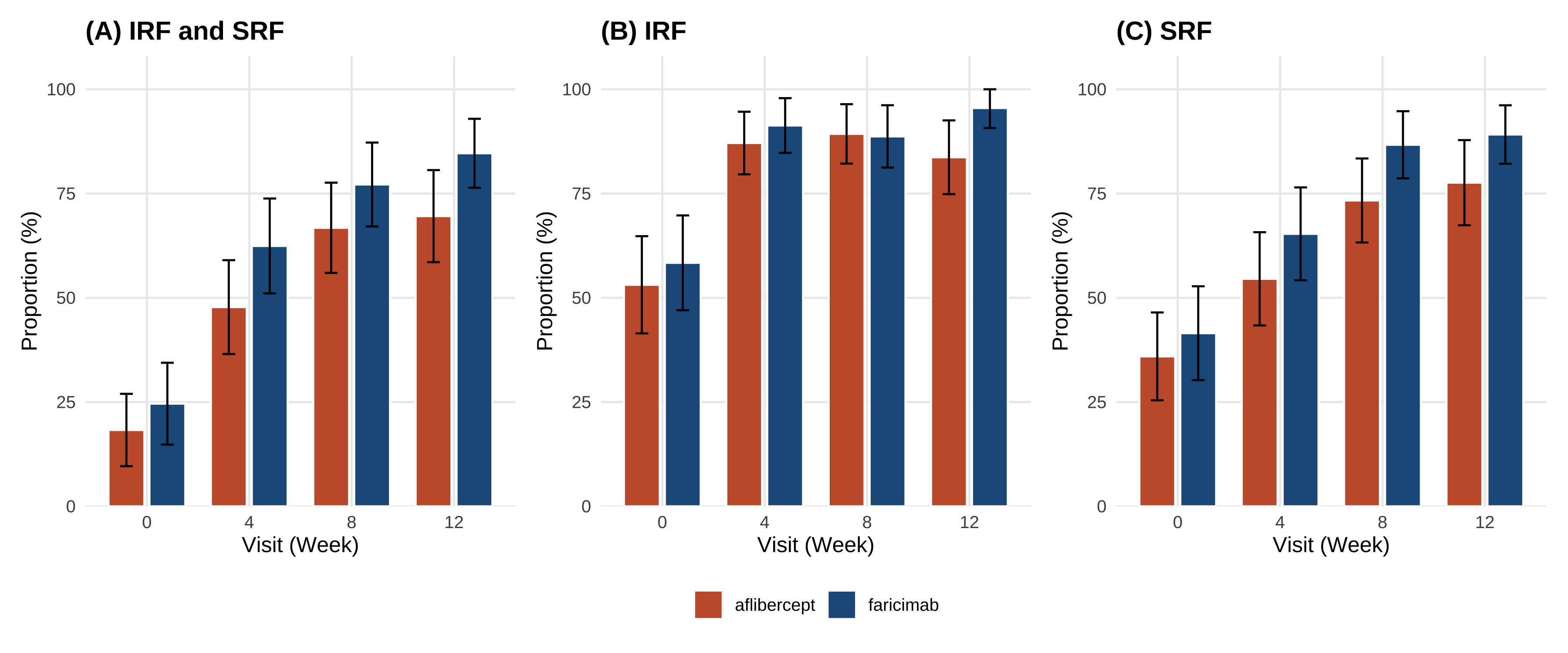
# Part 5:換你院內資料(含 PSM + ASMD) ```{r} #| label: setup-part5 #| include: false source ("_common.R" )library (readr)library (dplyr)library (tidyr)library (gtsummary)library (MatchIt)library (cobalt)library (mmrm)library (emmeans)library (ggplot2)library (patchwork)``` > 上半場你看到了:1329 個病人、24 個 stratum、漂亮的 paper 圖。 > > 下半場你會看到:**同樣的 pipeline、加上 PSM 處理院內 cohort 的非隨機分派、跑出可投稿的 Figure 1/2 草稿**。 - **PSM(propensity score matching)**:Austin 2011 *Multivariate Behavioral Research*[@austin2011propensity]、Stuart 2010 *Statistical Science*[ @stuart2010matching ] - **ASMD(absolute standardized mean difference)**:Austin 2009 *Statistics in Medicine*[ @austin2009smd ] - **MatchIt 套件**:Ho et al. 2011 *J Stat Softw*[ @ho2011matchit ] - **未測量混淆 sensitivity analysis(E-value)**:VanderWeele & Ding 2017 *Ann Intern Med*[ @vanderweele2017evalue ] 、限制與誤用見 Ioannidis 2019[ @ioannidis2019evaluelimits ] - **Target trial emulation 報告標準**:Hansford 2023 *JAMA Netw Open*[@hansford2023targettrial]、TARGET Statement 2025 *JAMA*[ @cashin2025target ] - **觀察性研究 adjusted analysis 解讀**:Agoritsas 2017 *JAMA* Users' Guide[ @agoritsas2017adjusted ] - **真實世界 faricimab cohort 範例**:Khanani 2024 TRUCKEE[ @khanani2024antivegf ] > AI 對 PSM 細節(caliper、ratio、common support、unmeasured confounding 估計)常會給「看起來像、其實不對」的答案。請以教材的參考程式碼為準,並回查上面的 ref 自行驗證。 ::: ## 任務 21:載入「假裝是你院內」的資料 `faricimab_my_hospital.csv` ,n = 180(faricimab 100 / aflibercept 80),region 全部 = `Asia-Pacific` 。> 請用 `readr::read_csv()` 讀 `data/faricimab_my_hospital_baseline.csv` 和 `data/faricimab_my_hospital_followup.csv` ,看欄位是否跟 trial 資料一致。 > > 回答之後,**請等我看過教材的「參考程式碼」再執行**——課堂上同學要跑同一份 code 結果才能對得上。 ```{r} #| label: load-mh # ── 前置(可單獨執行):套件 + 資料 ── library (readr); library (dplyr)<- read_csv ("data/faricimab_my_hospital_baseline.csv" ,show_col_types = FALSE )<- read_csv ("data/faricimab_my_hospital_followup.csv" ,show_col_types = FALSE )glimpse (mh_baseline)``` ```{r} #| label: glimpse-mh-fu glimpse (mh_followup)``` ```{r} #| label: mh-counts |> count (arm)``` > 詳細欄位定義在 [ `data/data_dictionary.md` ](https://github.com/htlin222/roche-vabysmo-rwe-workshop/blob/main/data/data_dictionary.md) 。 > **想做你自己的院內 cohort?把資料整成這個 schema、放進 `data/`、改下面的檔名就好。** ### 為什麼院內資料**必須**先做 PSM? | 方法 | 概念 | 何時用 | |---|---|---| | **Propensity score matching (PSM)** | 算每個病人「被分到 faricimab 的傾向分數」,然後 1:1 配對讓兩組分布相似 | n 中等(100–500),interpret 容易,本書範例 | | **Inverse probability of treatment weighting (IPTW)** | 每個病人加權,讓全 cohort 模擬隨機 | n 大、想保留樣本數時 | [ @stuart2010matching ] 。- **propensity score** = 「給定 baseline 共變項,被分到 treatment 組的機率」,通常用 logistic regression 估計- **caliper** = 配對時兩人傾向分數差距的上限;常用 0.2 × SD(logit(propensity))- **ratio** = 配對比例(1:1、1:2、1:k);本書用 1:1 nearest neighbor## 任務 22:診斷 baseline 不平衡(PSM 前的 ASMD) > 我有一個 R data frame `mh_baseline` ,欄位 patient_id, arm (faricimab/aflibercept), age, sex, bcva_baseline, cst_baseline, irf_baseline, srf_baseline, bcva_strat, lld_strat。請用 `cobalt::bal.tab()` 算每個共變項的 absolute standardized mean difference (ASMD),threshold = 0.1,並幫我解讀哪些變項不平衡。 ### 參考程式碼 ```{r} #| label: psm-pre-asmd # ── 前置(可單獨執行):套件 + 資料 ── library (readr); library (dplyr); library (cobalt)# treat / factor 一起在讀檔時建好,往後每段沿用同一份 mh_baseline <- read_csv ("data/faricimab_my_hospital_baseline.csv" ,show_col_types = FALSE ) |> mutate (treat = if_else (arm == "faricimab" , 1 L, 0 L),sex = factor (sex),bcva_strat = factor (bcva_strat),lld_strat = factor (lld_strat)<- c ("age" , "sex" , "bcva_baseline" , "cst_baseline" ,"irf_baseline" , "srf_baseline" , "bcva_strat" , "lld_strat" )<- bal.tab (reformulate (covariates, response = "treat" ),data = mh_baseline,estimand = "ATT" ,thresholds = c (m = 0.1 ),un = TRUE ``` - **|ASMD| < 0.1** ✅ 平衡,不需要 adjust- **0.1 ≤ |ASMD| < 0.25** ⚠️ 輕微不平衡,建議 adjust- **|ASMD| ≥ 0.25** ❌ 嚴重不平衡,必定要 PSM 或在 model 裡 adjust## 任務 23:跑 1:1 nearest neighbor PSM > 請用 `MatchIt::matchit()` 做 1:1 nearest neighbor PSM,treatment 是 faricimab vs aflibercept,共變項 age, sex, bcva_baseline, cst_baseline, irf_baseline, srf_baseline, bcva_strat, lld_strat,distance 用 logistic regression、caliper = 0.2、ratio = 1。配對完拿 `match.data()` 。 ### 參考程式碼 ```{r} #| label: psm-fit # ── 前置(可單獨執行):套件 + 資料 ── library (readr); library (dplyr); library (MatchIt)<- read_csv ("data/faricimab_my_hospital_baseline.csv" ,show_col_types = FALSE ) |> mutate (treat = if_else (arm == "faricimab" , 1 L, 0 L),sex = factor (sex), bcva_strat = factor (bcva_strat),lld_strat = factor (lld_strat))<- read_csv ("data/faricimab_my_hospital_followup.csv" ,show_col_types = FALSE )set.seed (20260530 )<- matchit (~ age + sex + bcva_baseline + cst_baseline + + srf_baseline + bcva_strat + lld_strat,data = mh_baseline,method = "nearest" ,distance = "glm" ,ratio = 1 ,caliper = 0.2 summary (m_out)``` ```{r} #| label: psm-matched-data <- match.data (m_out) |> as_tibble ()cat ("配對後樣本數:" , nrow (mh_matched),"(faricimab:" , sum (mh_matched$ treat == 1 ),"aflibercept:" , sum (mh_matched$ treat == 0 ), ") \n " )<- mh_followup |> semi_join (mh_matched, by = "patient_id" )cat ("配對後 follow-up rows:" , nrow (mh_matched_followup), " \n " )``` ## 任務 24:配對後重算 ASMD + Love plot > 請用 `cobalt::bal.tab()` 算配對後的 ASMD,並用 `cobalt::love.plot()` 畫前後對比的 Love plot(threshold 線 0.1)。 ### 參考程式碼 ```{r} #| label: psm-post-asmd # ── 前置(可單獨執行):套件 + 資料 ── library (cobalt)# ⚠️ 沿用前面任務的物件:m_out(請先跑完任務23,本段不重算) <- bal.tab (m_out, thresholds = c (m = 0.1 ), un = TRUE )``` ```{r} #| label: fig-love-plot #| fig-cap: "Love plot — PSM 前後 ASMD 對比;垂直線是 0.1 平衡門檻" #| fig-width: 8 #| fig-height: 5 love.plot (binary = "std" ,threshold = 0.1 ,abs = TRUE ,var.order = "unadjusted" ,colors = c ("#C75D38" , "#1F5C8B" ),shapes = c ("circle filled" , "triangle filled" ),sample.names = c ("配對前 (Unadjusted)" , "配對後 (Matched)" ),title = "ASMD: Before vs After 1:1 PSM" + theme (legend.position = "bottom" )``` 1. **大部分變項 ASMD 從 > 0.1 掉到 < 0.1**(紅圈 → 藍三角)2. **沒有任何變項配對後反而更不平衡**3. 樣本縮水可接受(通常掉 10–30%)## 任務 25:把 Part 2/3/4 的 pipeline 套到 matched cohort ### 5.2.1 Table 1(unmatched — 顯示原始 cohort 的不平衡) ```{r} #| label: mh-table1 # ── 前置(可單獨執行):套件 + 資料 ── library (readr); library (dplyr); library (gtsummary)<- read_csv ("data/faricimab_my_hospital_baseline.csv" ,show_col_types = FALSE )|> select (arm, age, sex, region, bcva_baseline, cst_baseline,|> tbl_summary (by = arm,statistic = list (all_continuous () ~ "{mean} ({sd})" ,all_categorical () ~ "{n} ({p}%)" ),digits = list (all_continuous () ~ 1 )|> add_overall () |> modify_caption ("**Table 1 (My Hospital, unmatched).** Baseline characteristics, n=180" )``` ### 5.2.2 Figure 1(MMRM on matched cohort) ```{r} #| label: mh-fig1 #| fig-cap: "Figure 1 (My Hospital, post-PSM matched cohort) — MMRM on matched cohort" #| fig-width: 11 #| fig-height: 5 # ── 前置(可單獨執行):套件 + 資料 ── library (dplyr); library (tidyr); library (mmrm); library (emmeans)library (ggplot2); library (patchwork)<- c ("faricimab" = "#1F5C8B" , "aflibercept" = "#C75D38" )# ⚠️ 沿用前面任務的物件:mh_matched、mh_matched_followup(請先跑完任務23,本段不重算) <- mh_matched_followup |> left_join (|> select (patient_id, arm, study, region,by = "patient_id" |> mutate (bcva_change = bcva - bcva_baseline,cst_change = cst - cst_baseline,visit = factor (week, levels = c (4 , 8 , 12 )),arm = factor (arm, levels = c ("aflibercept" , "faricimab" )),bcva_strat = factor (bcva_strat),lld_strat = factor (lld_strat)<- tryCatch (mmrm (bcva_change ~ arm + visit + arm: visit + bcva_strat + lld_strat + us (visit | patient_id),data = mh_fu_long |> filter (! is.na (bcva_change))),error = function (e) {mmrm (bcva_change ~ arm + visit + arm: visit + bcva_strat + lld_strat + cs (visit | patient_id),data = mh_fu_long |> filter (! is.na (bcva_change)))<- tryCatch (mmrm (cst_change ~ arm + visit + arm: visit + bcva_strat + lld_strat + us (visit | patient_id),data = mh_fu_long |> filter (! is.na (cst_change))),error = function (e) {mmrm (cst_change ~ arm + visit + arm: visit + bcva_strat + lld_strat + cs (visit | patient_id),data = mh_fu_long |> filter (! is.na (cst_change)))<- as.data.frame (emmeans (m_bcva_mh, ~ arm | visit)) |> mutate (week = as.numeric (as.character (visit)))<- as.data.frame (emmeans (m_cst_mh, ~ arm | visit)) |> mutate (week = as.numeric (as.character (visit)))<- function (df) {bind_rows (data.frame (arm = c ("aflibercept" , "faricimab" ),week = 0 , emmean = 0 , lower.CL = 0 , upper.CL = 0 ),|> select (arm, week, emmean, lower.CL, upper.CL)|> arrange (arm, week)<- ggplot (baseline_zero (emm_b),aes (x = week, y = emmean, colour = arm, group = arm)) + geom_line (linewidth = 1 ) + geom_point (size = 3 ) + geom_errorbar (aes (ymin = lower.CL, ymax = upper.CL), width = 0.4 ) + scale_colour_manual (values = arm_colours, name = NULL ) + scale_x_continuous (breaks = c (0 , 4 , 8 , 12 )) + labs (title = "(A) BCVA — My Hospital (post-PSM)" ,x = "Time (Weeks)" , y = "Adjusted Mean BCVA Change \n (Letters)" )<- ggplot (baseline_zero (emm_c),aes (x = week, y = emmean, colour = arm, group = arm)) + geom_line (linewidth = 1 ) + geom_point (size = 3 ) + geom_errorbar (aes (ymin = lower.CL, ymax = upper.CL), width = 0.4 ) + scale_colour_manual (values = arm_colours, name = NULL ) + scale_x_continuous (breaks = c (0 , 4 , 8 , 12 )) + labs (title = "(B) CST — My Hospital (post-PSM)" ,x = "Time (Weeks)" , y = "Adjusted Mean CST Change \n (μm)" )+ p_c + plot_layout (guides = "collect" ) & theme (legend.position = "bottom" )``` - 走勢與 paper 一致:CST 兩 arm 都急速下降,faricimab 略多- CI 寬約 √(1329/n_matched) 倍- PSM 後估計值是「近似 ATT」(average treatment effect on the treated),論文要寫清楚### 5.2.3 Figure 2(CMH on matched cohort) ```{r} #| label: mh-fig2 #| fig-cap: "Figure 2 (My Hospital, post-PSM) — CMH-weighted absence proportions on matched cohort" #| fig-width: 12 #| fig-height: 5 # ── 前置(可單獨執行):套件 + 資料 ── library (dplyr); library (tidyr); library (ggplot2); library (patchwork)<- c ("faricimab" = "#1F5C8B" , "aflibercept" = "#C75D38" )# ⚠️ 沿用前面任務的物件:mh_matched、mh_matched_followup(請先跑完任務23,本段不重算) <- function (data, outcome_col,arm_col = "arm" ,strata_cols = c ("bcva_strat" , "lld_strat" )) {<- data |> filter (! is.na (.data[[outcome_col]])) |> mutate (stratum = do.call (paste, c (across (all_of (strata_cols)), sep = "|" )))<- d |> group_by (stratum, !! sym (arm_col)) |> summarise (n = n (), x = sum (.data[[outcome_col]]), p = x / n, .groups = "drop" )<- levels (factor (per_stratum[[arm_col]]))<- per_stratum |> select (stratum, !! sym (arm_col), n) |> pivot_wider (names_from = !! sym (arm_col), values_from = n, values_fill = 0 ) |> mutate (w = (.data[[arms[1 ]]] * .data[[arms[2 ]]]) / pmax (.data[[arms[1 ]]] + .data[[arms[2 ]]], 1 )) |> filter (.data[[arms[1 ]]] > 0 & .data[[arms[2 ]]] > 0 ) |> select (stratum, w)|> inner_join (ws, by = "stratum" ) |> group_by (!! sym (arm_col)) |> summarise (p_hat = sum (w * p) / sum (w),se = sqrt (sum (w^ 2 * p * (1 - p) / pmax (n, 1 ))) / sum (w),.groups = "drop" |> mutate (lower = pmax (p_hat - 1.96 * se, 0 ),upper = pmin (p_hat + 1.96 * se, 1 ))<- mh_matched_followup |> left_join (|> select (patient_id, arm, bcva_strat, lld_strat,by = "patient_id" |> mutate (abs_irf = if_else (is.na (irf), NA , as.integer (irf == 0 )),abs_srf = if_else (is.na (srf), NA , as.integer (srf == 0 )),abs_both = if_else (is.na (irf) | is.na (srf), NA ,as.integer (irf == 0 & srf == 0 )),arm = factor (arm, levels = c ("aflibercept" , "faricimab" ))<- mh_matched |> mutate (week = 0 L,abs_irf = as.integer (irf_baseline == 0 ),abs_srf = as.integer (srf_baseline == 0 ),abs_both = as.integer (irf_baseline == 0 & srf_baseline == 0 ),arm = factor (arm, levels = c ("aflibercept" , "faricimab" ))|> select (patient_id, arm, bcva_strat, lld_strat,<- bind_rows (|> select (patient_id, arm, bcva_strat, lld_strat,<- expand.grid (outcome = c ("abs_irf" , "abs_srf" , "abs_both" ),wk = c (0 , 4 , 8 , 12 ),stringsAsFactors = FALSE |> rowwise () |> mutate (res = list (cmh_weighted_proportion (|> filter (week == wk),outcome_col = outcome|> ungroup () |> :: unnest (res) |> rename (week = wk)<- function (out_col, ttl) {<- mh_results |> filter (outcome == out_col)ggplot (dat, aes (x = factor (week), y = p_hat * 100 , fill = arm)) + geom_col (position = position_dodge (width = 0.8 ),width = 0.7 , colour = "white" ) + geom_errorbar (aes (ymin = lower * 100 , ymax = upper * 100 ),position = position_dodge (width = 0.8 ), width = 0.25 ) + scale_fill_manual (values = arm_colours, name = NULL ) + scale_y_continuous (limits = c (0 , 100 ),expand = expansion (mult = c (0 , 0.08 ))) + labs (title = ttl, x = "Visit (Week)" , y = "Proportion (%)" ) + theme (legend.position = "bottom" )make_mh_panel ("abs_both" , "(A) IRF and SRF" ) | make_mh_panel ("abs_irf" , "(B) IRF" ) | make_mh_panel ("abs_srf" , "(C) SRF" )) + plot_layout (guides = "collect" ) & theme (legend.position = "bottom" )``` ## 任務 26:討論 — 你院內資料的 paper 該怎麼寫? > 我用 n=180 的院內 cohort、配對後做 1:1 PSM 跑出和 TENAYA/LUCERNE 同方向的結果,但 95% CI 寬很多。如果我要把這個結果投 Ophthalmology 這類期刊,我應該:(1)強調什麼?(2)reviewer 會質疑什麼?(3)下一步該怎麼處理 limitation?請給我 3 段建議文字。 > > (提醒:AI 給的論文寫法**會幻想 reviewer 意見**,請對照真實期刊的最新 RWE methodological standard 自行驗證。) 1. **Power 不足** → 解法:聯院 / 多中心、或定位成 hypothesis-generating2. **單一族群(Asia-Pacific)** → 解法:明確說 generalizability 限於該族群3. **PSM 把哪些人排除掉了?** → 解法:附 unmatched vs matched ASMD 對比表(Love plot)、報告 effective sample size[ @austin2009smd ] 4. **未測量混淆(unmeasured confounding)** → 解法:sensitivity analysis(E-value[ @vanderweele2017evalue; @ioannidis2019evaluelimits ] 、negative control outcome)5. **觀察期短(12 週)** → 解法:拉長到 48 / 60 / 108 週,引用 paper 的 long-term data 對比6. **是不是隨便找 cohort?** → 解法:用 **target trial emulation** framework 描述設計、follow TARGET / Hansford 2023 報告 checklist[ @cashin2025target; @hansford2023targettrial ] ## 任務 27:你回院後的 checklist ### Step 1:找院內 IT 撈 cohort - 年齡、性別、區域(如果跨院)- index 日期(首次注射日)- index 日後 4/8/12 週的 BCVA、OCT CST- index 日後 4/8/12 週的 OCT 報告(IRF/SRF presence)- baseline 共變項:合併症、過去打過幾針、是否雙眼…(PSM 共變項清單越完整越好)」### Step 2:IRB 申請 - 一般院內 retrospective chart review,預期可走 expedited review- 把這份 csv schema 與本書 Quarto 連結貼進 protocol,reviewer 看就懂### Step 3:把 csv 放進 `data/`、改本書 `_quarto.yml` 的 title → render ```r :: quarto_render ()``` `_book/` 裡就是「**用你院內資料做出的論文 draft**」。### Step 4:拿給 Shao 看(眨眼) 1. 院內 RWE 沒有隨機分派 → **必須先做 PSM 或 IPTW**,否則 reviewer 退稿2. PSM 三步驟:算 propensity score → caliper-restricted nearest neighbor matching → 重算 ASMD 確認 < 0.13. **5.2.2(MMRM)和 5.2.3(CMH)使用 matched cohort**,Table 1 同時呈現 unmatched 與 matched4. PSM 後估計的是 ATT(不是 RCT 的 ATE),論文要寫清楚5. 同一份 pipeline + 換 csv 路徑就能跑,但 Power 與 generalizability 限制要誠實寫