# ── 前置(可單獨執行):套件 + 資料 ──
library(readr); library(dplyr); library(tidyr)
library(ggplot2); library(patchwork)
arm_colours <- c("faricimab" = "#1F5C8B", "aflibercept" = "#C75D38")
baseline <- read_csv("data/faricimab_baseline.csv", show_col_types = FALSE)
followup <- read_csv("data/faricimab_followup.csv", show_col_types = FALSE)
fu_with_strata <- followup |>
  left_join(
    baseline |> select(patient_id, arm, study, bcva_strat, lld_strat, region,
                       irf_baseline, srf_baseline),
    by = "patient_id"
  ) |>
  mutate(
    abs_irf  = if_else(is.na(irf), NA, as.integer(irf == 0)),
    abs_srf  = if_else(is.na(srf), NA, as.integer(srf == 0)),
    abs_both = if_else(is.na(irf) | is.na(srf), NA,
                       as.integer(irf == 0 & srf == 0)),
    arm = factor(arm, levels = c("aflibercept","faricimab"))
  )

# 加一筆 baseline (week=0) 的 absence rate
baseline_abs <- baseline |>
  mutate(
    week = 0L,
    abs_irf  = as.integer(irf_baseline == 0),
    abs_srf  = as.integer(srf_baseline == 0),
    abs_both = as.integer(irf_baseline == 0 & srf_baseline == 0),
    arm = factor(arm, levels = c("aflibercept","faricimab"))
  ) |>
  select(patient_id, arm, study, bcva_strat, lld_strat, region,
         week, abs_irf, abs_srf, abs_both)

fu_with_strata <- bind_rows(
  baseline_abs,
  fu_with_strata |> select(patient_id, arm, study, bcva_strat, lld_strat, region,
                           week, abs_irf, abs_srf, abs_both)
)4 Part 4:Figure 2 — CMH-weighted absence proportions
預計時間:30 分鐘。 deliverable:三張 absence proportion bar chart(IRF / SRF / IRF+SRF),對得起 paper Figure 2。
📚 CMH / stratified analysis 方法學引用
- CMH 原始:Mantel & Haenszel 19591
- 稀疏分層的方差估計:Greenland & Robins 19852
- MH 在 RCT 中的角色與最新觀點:Qiu et al. 2025 Biometrics3
- 加權選擇(minimum-risk vs CMH):Mehrotra & Railkar 20004
- 多分層因子的 adjustment:Kahan & Morris 20135、Agoritsas 2017 JAMA6
AI 對 CMH 權重公式(hypergeometric 還是 sample-size weights)、空 stratum 處理、以及加權 vs unstratified 之間的差異經常給錯。Cheung 2025 paper 採 CMH-weighted proportion,本書範例對齊 paper、並在小 stratum 自動 drop 掉。
🚀 一鍵 Prompt:整章一次跑完
我有 R data frame
baseline和followup(已合併好),想做 paper Figure 2:分別在 week 4、8、12 算「absence of IRF」、「absence of SRF」、「absence of both」這三個 outcome 的比例,分 arm,並且 CMH-weighted by 分層因子(study × bcva_strat × lld_strat × region)。請給我 R code:
- 寫一個 helper 函數
cmh_weighted_proportion(data, outcome, arm_col, strata_cols),回傳 weighted proportion + 95% CI per arm- 對 IRF absence、SRF absence、IRF+SRF absence 各跑 4 個 visit (0/4/8/12)
- 用
mantelhaen.test()算 stratified test 的 p value (faricimab vs aflibercept)- 用 ggplot 三個 panel 畫 bar chart,y 是 %,x 是 visit,fill by arm,加 error bar,星號標 p < 0.05
加中文註解。我用 Posit.Cloud。
4.1 任務 16:什麼是 stratified analysis?為什麼要 weight?
📋 複製這段話,貼給 AI(🆕 開新對話):
請用「給沒學過統計的眼科醫師聽」的方式,100 字內解釋: 1. 什麼是 stratified analysis? 2. 為什麼比較兩 arm 的「比例」要 stratify by 隨機分層因子(study × baseline severity × region)? 3. CMH (Cochran-Mantel-Haenszel) test 在做什麼?
速記
📖 名詞|stratum / strata / 為何 24 個
- stratum(單) / strata(複)= 「同質子群」。本書用
study × bcva_strat × lld_strat × region共 4 個分層因子,levels 各 2/3/2/2 → 2 × 3 × 2 × 2 = 24 個 stratum - 每個 stratum 內,兩 arm 的人應該很像(隨機分派 + 分層)→ 比較才公平
- 如果 stratum 太多、每格人數太少,CMH 估計會不穩 → Part 5 院內 n=180 時會看到這問題,需要合併分層
4.2 任務 17:建立 wide-by-visit 的資料
把 followup 接上 baseline 的分層因子,並算出每個 visit 的 absence indicator。
4.3 任務 18:先用 base R 的 mantelhaen.test() 看一下整體 p value
📋 複製這段話,貼給 AI(🆕 開新對話):
用 R 內建
mantelhaen.test()對 week 12 的「IRF and SRF both absent」outcome 做 stratified test:兩 arm 的差異,stratified by study × bcva_strat × lld_strat × region。
4.3.1 參考程式碼
# ── 前置(可單獨執行):套件 + 資料 ──
library(readr); library(dplyr); library(tidyr)
library(ggplot2); library(patchwork)
arm_colours <- c("faricimab" = "#1F5C8B", "aflibercept" = "#C75D38")
baseline <- read_csv("data/faricimab_baseline.csv", show_col_types = FALSE)
followup <- read_csv("data/faricimab_followup.csv", show_col_types = FALSE)
# ⚠️ 沿用前面任務的物件:fu_with_strata(請先跑完任務17,本段不重算)
cmh_test_at_week <- function(data, outcome_col, week_val) {
  d <- data |>
    filter(week == week_val) |>
    mutate(stratum = paste(study, bcva_strat, lld_strat, region, sep = "|")) |>
    filter(!is.na(.data[[outcome_col]]))
  arr <- xtabs(
    as.formula(paste0("~ arm + ", outcome_col, " + stratum")),
    data = d
  )
  # drop strata with empty cells in either arm
  good <- apply(arr, 3, function(m) all(rowSums(m) > 0) && all(colSums(m) > 0))
  arr <- arr[, , good, drop = FALSE]
  mantelhaen.test(arr, exact = FALSE)
}

cmh_test_at_week(fu_with_strata, "abs_both", 12)
    Mantel-Haenszel chi-squared test with continuity correction

data:  arr
Mantel-Haenszel X-squared = 20.965, df = 1, p-value = 4.678e-06
alternative hypothesis: true common odds ratio is not equal to 1
95 percent confidence interval:
 1.424213 2.399854
sample estimates:
common odds ratio
         1.848757
Tip
Mantel-Haenszel X-squared 越大、p 越小,代表「在分層之後,兩臂的差異仍顯著」。
4.4 任務 19:寫 helper 算 CMH-weighted proportion 與 95% CI
📋 複製這段話,貼給 AI(↩︎️ 續前對話):
請給我一個 R 函數
cmh_weighted_proportion(data, outcome_col, arm_col, strata_cols): 1. 對每個 (stratum × arm),算 proportion (events / n) 2. CMH 權重 w_k = (n_1k * n_2k) / (n_1k + n_2k) 3. 加權平均:p_hat_arm = Σ w_k * p_arm_k / Σ w_k 4. SE:sqrt(Σ w_k^2 * p * (1-p) / n) / Σ w_k 5. 回傳 tibble (arm, p_hat, se, lower, upper) 6. 跳過 stratum 中 n=0 的
4.4.1 參考程式碼
# ── 前置(可單獨執行):套件 + 資料 ──
library(readr); library(dplyr); library(tidyr)
library(ggplot2); library(patchwork)
arm_colours <- c("faricimab" = "#1F5C8B", "aflibercept" = "#C75D38")
baseline <- read_csv("data/faricimab_baseline.csv", show_col_types = FALSE)
followup <- read_csv("data/faricimab_followup.csv", show_col_types = FALSE)
# ⚠️ 沿用前面任務的物件:fu_with_strata(請先跑完任務17,本段不重算)
cmh_weighted_proportion <- function(data, outcome_col,
                                    arm_col = "arm",
                                    strata_cols = c("study","bcva_strat","lld_strat","region")) {
  d <- data |>
    filter(!is.na(.data[[outcome_col]])) |>
    mutate(stratum = do.call(paste, c(across(all_of(strata_cols)), sep = "|")))

  per_stratum <- d |>
    group_by(stratum, !!sym(arm_col)) |>
    summarise(
      n = n(),
      x = sum(.data[[outcome_col]]),
      p = x / n,
      .groups = "drop"
    )

  # 將每個 stratum pivot 成 (n_arm1, n_arm2),計算 CMH weight
  arms <- levels(factor(per_stratum[[arm_col]]))
  stopifnot(length(arms) == 2)

  ws <- per_stratum |>
    select(stratum, !!sym(arm_col), n) |>
    pivot_wider(names_from = !!sym(arm_col), values_from = n,
                values_fill = 0) |>
    mutate(w = (.data[[arms[1]]] * .data[[arms[2]]]) /
                pmax(.data[[arms[1]]] + .data[[arms[2]]], 1)) |>
    filter(.data[[arms[1]]] > 0 & .data[[arms[2]]] > 0) |>
    select(stratum, w)

  per_stratum |>
    inner_join(ws, by = "stratum") |>
    group_by(!!sym(arm_col)) |>
    summarise(
      p_hat = sum(w * p) / sum(w),
      se    = sqrt(sum(w^2 * p * (1 - p) / pmax(n, 1))) / sum(w),
      .groups = "drop"
    ) |>
    mutate(
      lower = pmax(p_hat - 1.96 * se, 0),
      upper = pmin(p_hat + 1.96 * se, 1)
    )
}

# Sanity check: faricimab vs aflibercept SRF absence at week 12
cmh_weighted_proportion(
  fu_with_strata |> filter(week == 12),
  outcome_col = "abs_srf"
)
# A tibble: 2 × 5
arm p_hat se lower upper
<fct> <dbl> <dbl> <dbl> <dbl>
1 aflibercept 0.790 0.0161 0.758 0.821
2 faricimab 0.892 0.0121 0.868 0.915對照 paper:faricimab 87.9% (85.4–90.4)、aflibercept 79.0% (76.0–82.1)。差 ~9 pp。
4.5 跑全部 outcome × visit × arm
# ── 前置(可單獨執行):套件 + 資料 ──
library(readr); library(dplyr); library(tidyr)
library(ggplot2); library(patchwork)
arm_colours <- c("faricimab" = "#1F5C8B", "aflibercept" = "#C75D38")
baseline <- read_csv("data/faricimab_baseline.csv", show_col_types = FALSE)
followup <- read_csv("data/faricimab_followup.csv", show_col_types = FALSE)
# ⚠️ 沿用前面任務的物件:fu_with_strata、cmh_weighted_proportion(請先跑完任務17、19,本段不重算)
all_results <- expand.grid(
  outcome = c("abs_irf", "abs_srf", "abs_both"),
  wk      = c(0, 4, 8, 12),
  stringsAsFactors = FALSE
) |>
  rowwise() |>
  mutate(
    res = list(
      cmh_weighted_proportion(
        fu_with_strata |> filter(week == wk),
        outcome_col = outcome
      )
    )
  ) |>
  ungroup() |>
  tidyr::unnest(res) |>
  rename(week = wk)

all_results
# A tibble: 24 × 7
outcome week arm p_hat se lower upper
<chr> <dbl> <fct> <dbl> <dbl> <dbl> <dbl>
1 abs_irf 0 aflibercept 0.520 0.0193 0.482 0.558
2 abs_irf 0 faricimab 0.574 0.0190 0.537 0.611
3 abs_srf 0 aflibercept 0.336 0.0178 0.301 0.371
4 abs_srf 0 faricimab 0.336 0.0180 0.300 0.371
5 abs_both 0 aflibercept 0.170 0.0142 0.142 0.198
6 abs_both 0 faricimab 0.189 0.0149 0.160 0.218
# ℹ 18 more rows加上 stratified p value:
get_p <- function(outcome_col, w) {
  if (w == 0) return(NA_real_)
  test <- tryCatch(
    cmh_test_at_week(fu_with_strata, outcome_col, w),
    error = function(e) NULL
  )
  if (is.null(test)) NA_real_ else test$p.value
}

p_table <- expand.grid(
  outcome = c("abs_irf", "abs_srf", "abs_both"),
  wk      = c(4, 8, 12),
  stringsAsFactors = FALSE
) |>
  rowwise() |>
  mutate(p = get_p(outcome, wk)) |>
  ungroup() |>
  rename(week = wk)

p_table
# A tibble: 9 × 3
outcome week p
<chr> <dbl> <dbl>
1 abs_irf 4 0.00634
2 abs_srf 4 0.00332
3 abs_both 4 0.000198
4 abs_irf 8 0.0284
5 abs_srf 8 0.0708
6 abs_both 8 0.0208
# ℹ 3 more rows4.6 任務 20:畫 Figure 2 — 三個 panel
📋 複製這段話,貼給 AI(↩︎️ 續前對話):
我有
all_results(outcome, week, arm, p_hat, lower, upper) 與p_table(outcome, week, p)。請用 ggplot2 + patchwork 畫三個 panel: 1. (A) Absence of IRF and SRF 2. (B) Absence of IRF 3. (C) Absence of SRF每個 panel 是 grouped bar chart(fill by arm,position dodge),y 軸 0–100%、加 error bar、p < 0.05 的 visit 加星號。
4.6.1 參考程式碼
# ── 前置(可單獨執行):套件 + 資料 ──
library(readr); library(dplyr); library(tidyr)
library(ggplot2); library(patchwork)
arm_colours <- c("faricimab" = "#1F5C8B", "aflibercept" = "#C75D38")
baseline <- read_csv("data/faricimab_baseline.csv", show_col_types = FALSE)
followup <- read_csv("data/faricimab_followup.csv", show_col_types = FALSE)
# ⚠️ 沿用前面任務的物件:all_results、p_table(請先跑完前面所有任務,本段不重算)
make_panel <- function(outcome_col, panel_title) {
  dat <- all_results |>
    filter(outcome == outcome_col) |>
    mutate(arm_lbl = factor(arm,
              levels = c("aflibercept","faricimab"),
              labels = c("Aflibercept Q8W (n=664)",
                         "Faricimab up to Q16W (n=665)")))
  ps <- p_table |> filter(outcome == outcome_col)

  ggplot(dat, aes(x = factor(week), y = p_hat * 100, fill = arm)) +
    geom_col(position = position_dodge(width = 0.8), width = 0.7,
             colour = "white") +
    geom_errorbar(aes(ymin = lower * 100, ymax = upper * 100),
                  position = position_dodge(width = 0.8),
                  width = 0.25) +
    geom_text(aes(label = round(p_hat * 100)),
              position = position_dodge(width = 0.8),
              vjust = 1.5, colour = "white", size = 3.2,
              fontface = "bold") +
    geom_text(
      data = ps |> filter(!is.na(p) & p < 0.05),
      aes(x = factor(week), y = 100, label = "*"),
      inherit.aes = FALSE, vjust = -0.2, size = 5
    ) +
    scale_fill_manual(values = arm_colours, name = NULL) +
    scale_y_continuous(limits = c(0, 100),
                       expand = expansion(mult = c(0, 0.08))) +
    labs(title = panel_title,
         x = "Visit (Week)",
         y = "Proportion of patients (%)") +
    theme(legend.position = "bottom")
}

p_irf_srf <- make_panel("abs_both", "(A) Absence of IRF and SRF")
p_irf     <- make_panel("abs_irf",  "(B) Absence of IRF")
p_srf     <- make_panel("abs_srf",  "(C) Absence of SRF")
(p_irf_srf | p_irf | p_srf) +
plot_layout(guides = "collect") &
theme(legend.position = "bottom")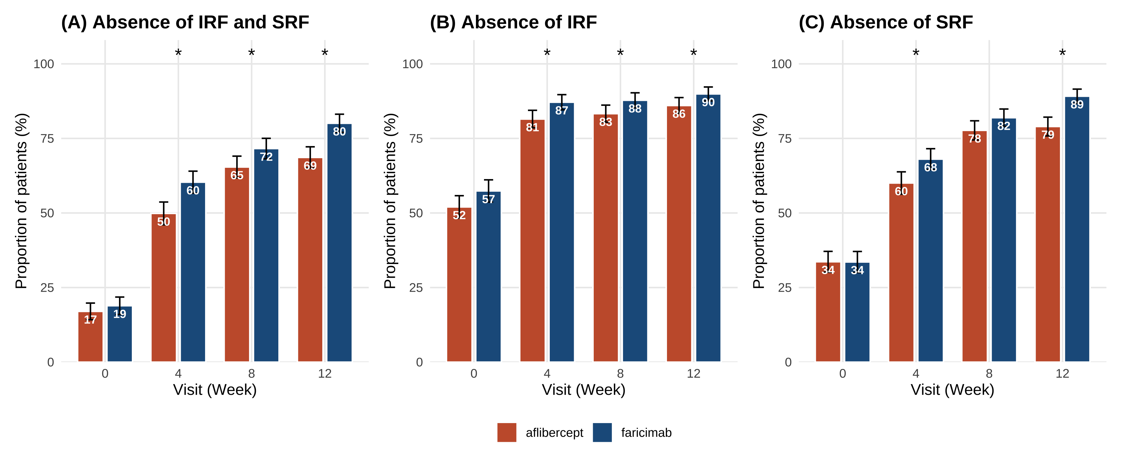
🎯 對得起 paper 嗎?
看 week 12: - 你的圖:IRF+SRF absence faricimab ~80% vs aflibercept ~68% - paper:IRF+SRF absence faricimab 77% vs aflibercept 67% - 都顯示 faricimab 顯著高,差約 10 pp ✅
本章重點
- 比例的「stratified analysis」= CMH weighted average
- base R
mantelhaen.test()給 p value;自寫 helper 給 weighted proportion + 95% CI - 同樣的 pipeline 可以用在任何二元 outcome(responder rate、AE rate、≥15 letter gain)
- 院內資料 stratum 太空時,函數會 drop 掉,proportion 仍可估
1.
Mantel N, Haenszel W. Statistical aspects of the analysis of data from retrospective studies of disease. Journal of the National Cancer Institute. 1959;22(4):719-748.
2.
Greenland S, Robins JM. Estimation of a common effect parameter from sparse follow-up data. Biometrics. 1985;41(1):55-68. doi:10.2307/2530643
3.
Qiu X, Qian Y, Yi J, et al. Clarifying the role of the Mantel–Haenszel risk difference estimator in randomized clinical trials. Biometrics. 2025;81(4):ujaf142. doi:10.1093/biomtc/ujaf142
4.
Mehrotra DV, Railkar R. Minimum risk weights for comparing treatments in stratified binomial trials. Statistics in Medicine. 2000;19(6):811-825. doi:10.1002/(SICI)1097-0258(20000330)19:6<811::AID-SIM390>3.0.CO;2-Z
5.
Kahan BC, Morris TP. Adjusting for multiple prognostic factors in the analysis of randomised trials. BMC Medical Research Methodology. 2013;13:99. doi:10.1186/1471-2288-13-99
6.
Agoritsas T, Merglen A, Shah ND, O’Donnell M, Guyatt GH. Adjusted analyses in studies addressing therapy and harm: Users’ guides to the medical literature. JAMA. 2017;317(7):748-759. doi:10.1001/jama.2016.20029