# 第五部分:統計檢定
```{r}
#| label: setup
#| include: false
source("_common.R")
```
本部分預計時間:30 分鐘
在第四部分,你已經學會畫出專業的圖表。現在我們要學習統計檢定 — 用數字證明你在圖表中看到的差異是否有意義。
::: {.callout-note collapse="true" title="一鍵 Prompt:整章一次跑完"}
> 我有兩份資料:
> - `patient_data.csv`:欄位 treatment(A/B)、age、gender(M/F)、los(住院天數)
> - `patient_data_for_survival.csv`:欄位 treatment(Drug_A/Drug_B)、age、gender、stage(I/II/III)、time(追蹤月數)、status(1=事件,0=設限)
>
> 請幫我一次完成以下統計分析:
>
> 1. 用 Shapiro-Wilk 檢定 los 的常態性,根據結果選擇 t-test 或 Wilcoxon test 比較兩組
> 2. 計算 Cohen's d 效應量,用白話文解讀結果
> 3. 檢查假設(Q-Q plot、Levene's test),說明不符合時的替代方法
> 4. 用卡方檢定比較兩組的性別比例
> 5. 用存活資料畫 Kaplan-Meier 曲線(含信賴區間和風險表),做 log-rank test
> 6. 跑 Cox 比例風險模型(treatment + age + gender + stage),整理成 gtsummary 表格
>
> 給我從讀取資料到產出所有結果的完整 script,加上中文註解。
:::
## 任務 20:讓 AI 選擇統計方法
📋 **複製這段話,貼給 AI:**
> 上傳 patient_data.csv 給 AI,然後問:
> 我想要比較兩組病人(treatment A vs B)的住院天數(los)有沒有顯著差異。我的資料存在 `patient_data` 裡面。
>
> 請幫我:
>
> 1. 依變項尺度、組數、配對與常態性,依教科書原則選擇最合適之統計,並簡要說明選擇理由。
> 2. 給我執行這個檢定的 R 程式碼,用內建的套件優先
> 3. 告訴我怎麼解讀結果
### 統計檢定選擇
```{r}
#| label: statistical-test
#| echo: true
#| message: false
#| warning: false
# 讀取資料
patient_data <- read.csv("patient_data.csv")
# 先檢查資料分佈
library(ggplot2)
# 檢視分佈圖(字型已由 _common.R 全域設定)
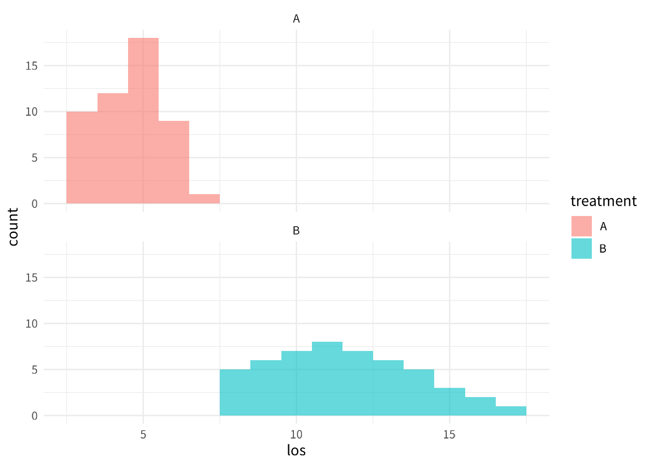
ggplot(patient_data, aes(x = los, fill = treatment)) +
geom_histogram(binwidth = 1, alpha = 0.6, position = "dodge") +
facet_wrap(~treatment, ncol = 1)
# Shapiro-Wilk 常態性檢定:p > 0.05 表示資料可能符合常態分佈
shapiro_a <- shapiro.test(patient_data$los[patient_data$treatment == "A"])
shapiro_b <- shapiro.test(patient_data$los[patient_data$treatment == "B"])

print("Shapiro-Wilk 常態性檢定結果:")
print(paste("A 組 p-value:", round(shapiro_a$p.value, 4)))
print(paste("B 組 p-value:", round(shapiro_b$p.value, 4)))
```
### 執行統計檢定
```{r}
#| label: t-test
#| echo: true
# 執行 t-test(假設資料符合常態分佈)
t_test_result <- t.test(los ~ treatment, data = patient_data)
print(t_test_result)
# 執行 Wilcoxon rank-sum test(無母數檢定)
wilcox_result <- wilcox.test(los ~ treatment, data = patient_data)
print(wilcox_result)
```
## 任務 21:解讀你的結果
📋 **把統計檢定的輸出複製起來,加上這段話貼給 AI:**
> 這是我的統計檢定結果:
> 【貼上輸出】
>
> 請用白話文解釋這個結果,包括:
>
> 1. 兩組有沒有顯著差異
> 2. p-value 是什麼意思
> 3. 這個結果在臨床上可能代表什麼
### 結果解讀
```{r}
#| label: interpret-results
#| echo: true
#| message: false
#| warning: false
# 載入必要套件
library(dplyr)

# 安裝並載入 broom 套件(用於整理統計結果)
if (!require(broom, quietly = TRUE)) {
  install.packages("broom", repos = "https://cloud.r-project.org/")
}
library(broom)

# 安裝並載入 effsize 套件(用於計算效應量)
if (!require(effsize, quietly = TRUE)) {
  install.packages("effsize", repos = "https://cloud.r-project.org/")
}
library(effsize)

# 整理結果摘要
result_summary <- patient_data %>%
  group_by(treatment) %>%
  summarise(
    n = n(),
    mean_los = mean(los),
    sd_los = sd(los),
    median_los = median(los),
    min_los = min(los),
    max_los = max(los)
  )

print("各組描述性統計:")
print(result_summary)
# 使用 broom::tidy() 整理 t-test 結果
t_test_tidy <- tidy(t_test_result)
print("T-test 結果(broom 整理後):")
print(t_test_tidy)
# 使用 broom::tidy() 整理 Wilcoxon 結果
wilcox_tidy <- tidy(wilcox_result)
print("Wilcoxon test 結果(broom 整理後):")
print(wilcox_tidy)
# 計算效應量(Cohen's d)
cohen_d <- cohen.d(los ~ treatment, data = patient_data)
print(paste("效應量 (Cohen's d):", round(cohen_d$estimate, 3)))
# 解釋
if (t_test_result$p.value < 0.05) {
  print("結論:兩組在統計上有顯著差異 (p < 0.05)")
  print(paste("B 組的平均住院天數比 A 組多約",
              round(diff(result_summary$mean_los), 1), "天"))
} else {
  print("結論:兩組在統計上無顯著差異 (p >= 0.05)")
}
```
### 產出純文字報告
```{r}
#| label: export-report
#| echo: true
#| message: false
#| warning: false
# 方法一:使用 sink() 將所有輸出導向檔案
sink("report.txt")

cat("=" %>% rep(60) %>% paste(collapse = ""), "\n")
cat("        統計分析報告:兩組治療住院天數比較\n")
cat("=" %>% rep(60) %>% paste(collapse = ""), "\n")
cat("報告產生時間:", format(Sys.time(), "%Y-%m-%d %H:%M:%S"), "\n\n")

cat("-" %>% rep(60) %>% paste(collapse = ""), "\n")
cat("一、描述性統計\n")
cat("-" %>% rep(60) %>% paste(collapse = ""), "\n")
print(result_summary)

cat("\n")
cat("-" %>% rep(60) %>% paste(collapse = ""), "\n")
cat("二、常態性檢定(Shapiro-Wilk Test)\n")
cat("-" %>% rep(60) %>% paste(collapse = ""), "\n")
cat("A 組 p-value:", round(shapiro_a$p.value, 4), "\n")
cat("B 組 p-value:", round(shapiro_b$p.value, 4), "\n")
if (shapiro_a$p.value >= 0.05 & shapiro_b$p.value >= 0.05) {
  cat("結論:兩組資料均符合常態分佈假設\n")
} else {
  cat("結論:至少一組資料不符合常態分佈假設\n")
}

cat("\n")
cat("-" %>% rep(60) %>% paste(collapse = ""), "\n")
cat("三、統計檢定結果\n")
cat("-" %>% rep(60) %>% paste(collapse = ""), "\n")

cat("\n【T-test 結果】\n")
cat("檢定方法:", t_test_tidy$method, "\n")
cat("t 統計量:", round(t_test_tidy$statistic, 4), "\n")
cat("自由度:", round(t_test_tidy$parameter, 2), "\n")
cat("p-value:", format(t_test_tidy$p.value, digits = 4, scientific = FALSE), "\n")
cat("95% 信賴區間:[", round(t_test_tidy$conf.low, 2), ", ",
    round(t_test_tidy$conf.high, 2), "]\n")
cat("兩組平均差異:", round(t_test_tidy$estimate1 - t_test_tidy$estimate2, 2), "天\n")

cat("\n【Wilcoxon Rank-Sum Test 結果】\n")
cat("檢定方法:", wilcox_tidy$method, "\n")
cat("W 統計量:", wilcox_tidy$statistic, "\n")
cat("p-value:", format(wilcox_tidy$p.value, digits = 4, scientific = FALSE), "\n")

cat("\n")
cat("-" %>% rep(60) %>% paste(collapse = ""), "\n")
cat("四、效應量\n")
cat("-" %>% rep(60) %>% paste(collapse = ""), "\n")
cat("Cohen's d:", round(cohen_d$estimate, 3), "\n")
cat("效應量大小:", as.character(cohen_d$magnitude), "\n")
cat("\n效應量解讀標準:\n")
cat("  |d| < 0.2:微小效應\n")
cat("  0.2 <= |d| < 0.5:小效應\n")
cat("  0.5 <= |d| < 0.8:中效應\n")
cat("  |d| >= 0.8:大效應\n")

cat("\n")
cat("-" %>% rep(60) %>% paste(collapse = ""), "\n")
cat("五、結論\n")
cat("-" %>% rep(60) %>% paste(collapse = ""), "\n")
if (t_test_result$p.value < 0.05) {
  cat("統計結論:兩組住院天數有顯著差異 (p < 0.05)\n")
  cat("臨床意義:B 組的平均住院天數比 A 組多約",
      round(diff(result_summary$mean_los), 1), "天\n")
} else {
  cat("統計結論:兩組住院天數無顯著差異 (p >= 0.05)\n")
  cat("臨床意義:目前證據不足以證明兩種治療在住院天數上有差異\n")
}

cat("\n")
cat("=" %>% rep(60) %>% paste(collapse = ""), "\n")
cat("報告結束\n")
cat("=" %>% rep(60) %>% paste(collapse = ""), "\n")

sink()  # 關閉 sink,恢復正常輸出

# 確認檔案已產生
cat("報告已儲存至 report.txt\n")
cat("檔案大小:", file.info("report.txt")$size, "bytes\n")
# 顯示報告內容預覽
cat("\n--- 報告內容預覽 ---\n")
cat(readLines("report.txt", n = 20), sep = "\n")
cat("...\n")
```
## 任務 22:檢查假設
📋 **複製這段話,貼給 AI:**
> 剛剛的統計檢定有什麼前提假設?我要怎麼用 R 檢查我的資料有沒有符合這些假設?如果不符合,有什麼替代方法?
### 假設檢驗
```{r}
#| label: check-assumptions
#| echo: true
#| message: false
#| warning: false
# 1. 檢查常態性
if (!require(car, quietly = TRUE)) {
install.packages("car", repos = "https://cloud.r-project.org/")
library(car)
}
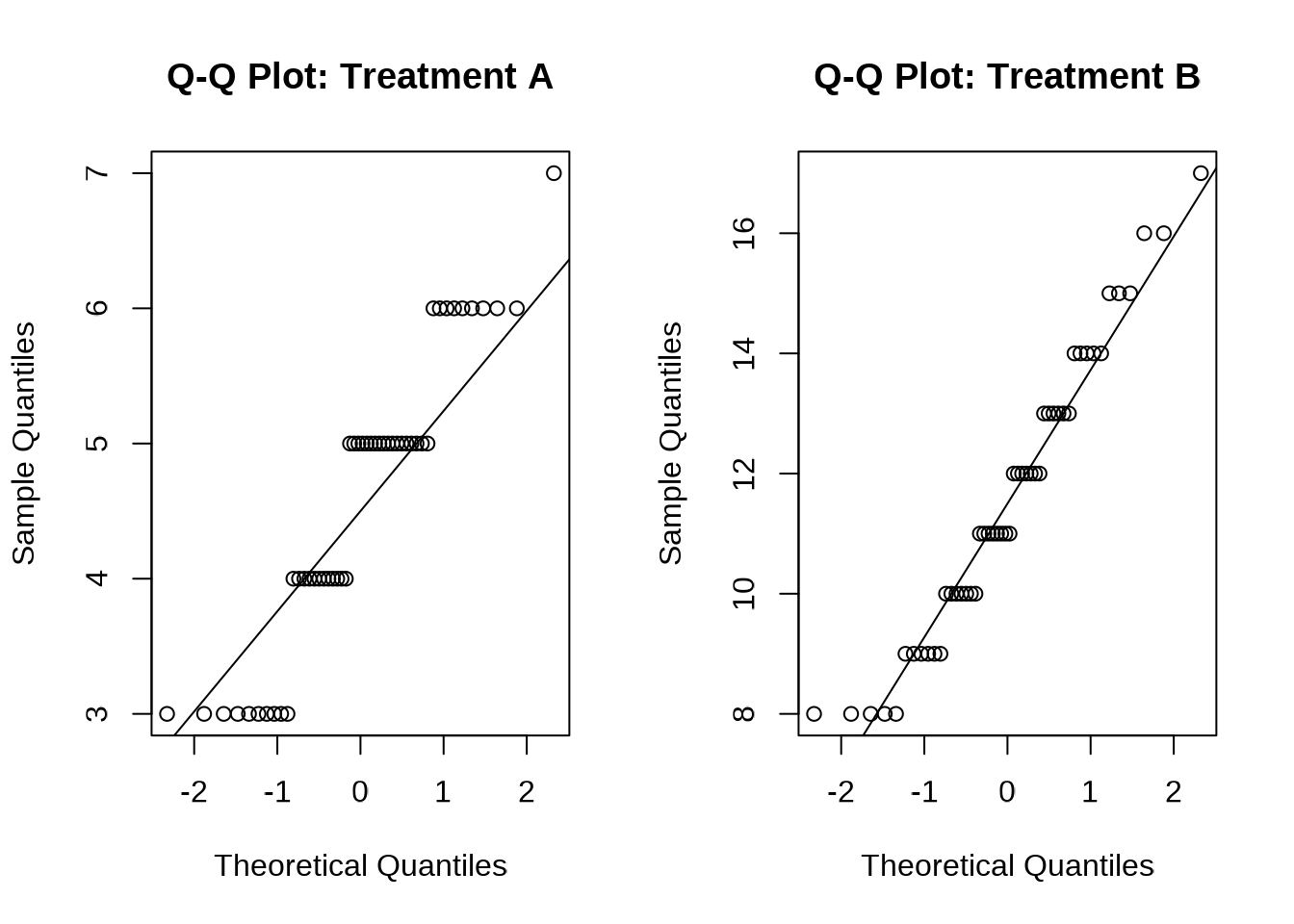
# Q-Q plot
par(mfrow = c(1, 2))
qqnorm(patient_data$los[patient_data$treatment == "A"], main = "Q-Q Plot: Treatment A")
qqline(patient_data$los[patient_data$treatment == "A"])
qqnorm(patient_data$los[patient_data$treatment == "B"], main = "Q-Q Plot: Treatment B")
qqline(patient_data$los[patient_data$treatment == "B"])
# 2. 檢查變異數同質性
levene_result <- leveneTest(los ~ treatment, data = patient_data)
print("Levene's Test for Homogeneity of Variance:")
print(levene_result)
# 3. 根據假設檢驗結果選擇適當方法
if (shapiro_a$p.value < 0.05 | shapiro_b$p.value < 0.05) {
  print("建議:資料不符合常態分佈,應使用 Wilcoxon rank-sum test")
} else if (levene_result$`Pr(>F)`[1] < 0.05) {
  print("建議:變異數不同質,應使用 Welch's t-test")
  welch_result <- t.test(los ~ treatment, data = patient_data, var.equal = FALSE)
  print(welch_result)
} else {
  print("建議:資料符合所有假設,可使用 Student's t-test")
}
```
## 任務 23:類別變數的比較
📋 **複製這段話,貼給 AI:**
> 我想要看 treatment(A vs B)和 gender(M vs F)有沒有關聯。也就是說,A 組和 B 組的男女比例有沒有不同。
>
> 請給我適當的統計檢定程式碼,並教我怎麼解讀。
### 類別變數檢定
```{r}
#| label: categorical-test
#| echo: true
# 建立列聯表
contingency_table <- table(patient_data$treatment, patient_data$gender)
print("列聯表:")
print(contingency_table)
# 加上比例
prop_table <- prop.table(contingency_table, margin = 1) * 100
print("各組性別比例(%):")
print(round(prop_table, 1))
# 執行卡方檢定
chisq_result <- chisq.test(contingency_table)
print("卡方檢定結果:")
print(chisq_result)
# Fisher's exact test(適用於小樣本)
fisher_result <- fisher.test(contingency_table)
print("Fisher's exact test:")
print(fisher_result)
# 解讀結果
if (chisq_result$p.value < 0.05) {
  print("結論:兩組的性別分佈有顯著差異")
} else {
  print("結論:兩組的性別分佈無顯著差異")
}
```
## 任務 24:存活分析 (Survival Analysis)
在臨床研究中,我們經常需要分析「時間到事件」的資料,例如:
- 病人從診斷到死亡的時間
- 從治療開始到疾病復發的時間
- 從手術到再住院的時間
這類分析稱為 **存活分析 (Survival Analysis)**,是臨床研究中非常重要的統計方法。
### 存活分析的特殊之處
存活分析資料有一個特點:**設限 (Censoring)**
- 有些病人在研究結束時還活著(我們不知道他們最終會活多久)
- 有些病人中途失聯(lost to follow-up)
- 這些「不完整」的觀察值不能直接丟掉,需要特殊處理
::: {.callout-important}
## 新資料集
從這裡開始,我們使用另一份資料 `patient_data_for_survival.csv`(已包含在課程資料中)。這份資料的欄位和之前的 `patient_data.csv` 不同:
- `time`:追蹤時間(月)
- `status`:事件狀態(1 = 事件發生,0 = 設限/未發生)
- `treatment`:治療組別(Drug_A 或 Drug_B)
- `stage`:癌症期別(I、II、III)
:::
📋 **複製這段話,貼給 AI:**
> 我有一組存活分析的資料(patient_data_for_survival.csv),包含追蹤時間(time)和事件狀態(status,1=事件發生,0=設限)。請幫我:
>
> 1. 畫出 Kaplan-Meier 存活曲線,比較兩組治療
> 2. 用 log-rank test 檢定兩組有沒有差異
> 3. 用白話文解釋結果
::: {.callout-tip collapse="true" title="進階:如何選擇存活分析方法?"}
| 問題 | 方法選擇 |
|------|----------|
| 是不是 time-to-event?不是就回傳統 GLM | |
| 有沒有互斥終點截斷這個事件? | competing risks(CIF + cause-specific / Fine-Gray) |
| 同一人會不會多次發生這個事件,而且「次數」重要? | recurrent events |
| 是否在講多個臨床狀態與轉移路徑? | multi-state |
| 暴露/關鍵 covariate 隨時間出現或改變,或需要先活一段時間才能算暴露? | time-dependent / trial emulation,防 immortal time |
| 入隊時間、離隊(censoring)、中心/醫師,是否明顯和預後相關或構成分群? | left truncation、IPCW / joint、cluster-robust 或 frailty |
:::
### 讀取存活分析資料
```{r}
#| label: survival-load-data
#| echo: true
#| message: false
#| warning: false
# 讀取存活分析資料
survival_data <- read.csv("patient_data_for_survival.csv")

# 檢視資料結構
str(survival_data)
# 查看前幾筆
head(survival_data)
# 確認事件分佈
table(survival_data$treatment, survival_data$status)
```
### Kaplan-Meier 存活分析
```{r}
#| label: survival-km
#| echo: true
#| message: false
#| warning: false
# 安裝並載入必要套件
if (!require(survival, quietly = TRUE)) {
  install.packages("survival", repos = "https://cloud.r-project.org/")
}
if (!require(ggsurvfit, quietly = TRUE)) {
  install.packages("ggsurvfit", repos = "https://cloud.r-project.org/")
}

library(survival)
library(ggsurvfit)

# 建立存活物件
# Surv(time, status) 會建立一個存活時間物件
# time = 追蹤時間, status = 事件是否發生 (1=是, 0=否/設限)
surv_obj <- Surv(time = survival_data$time, event = survival_data$status)

# 看看存活物件長什麼樣子
head(surv_obj, 10)
# 注意:數字後面的 "+" 表示該觀察值是 censored(設限)
```
### 繪製 Kaplan-Meier 存活曲線
```{r}
#| label: survival-km-plot
#| echo: true
#| message: false
#| warning: false
#| fig-width: 10
#| fig-height: 8
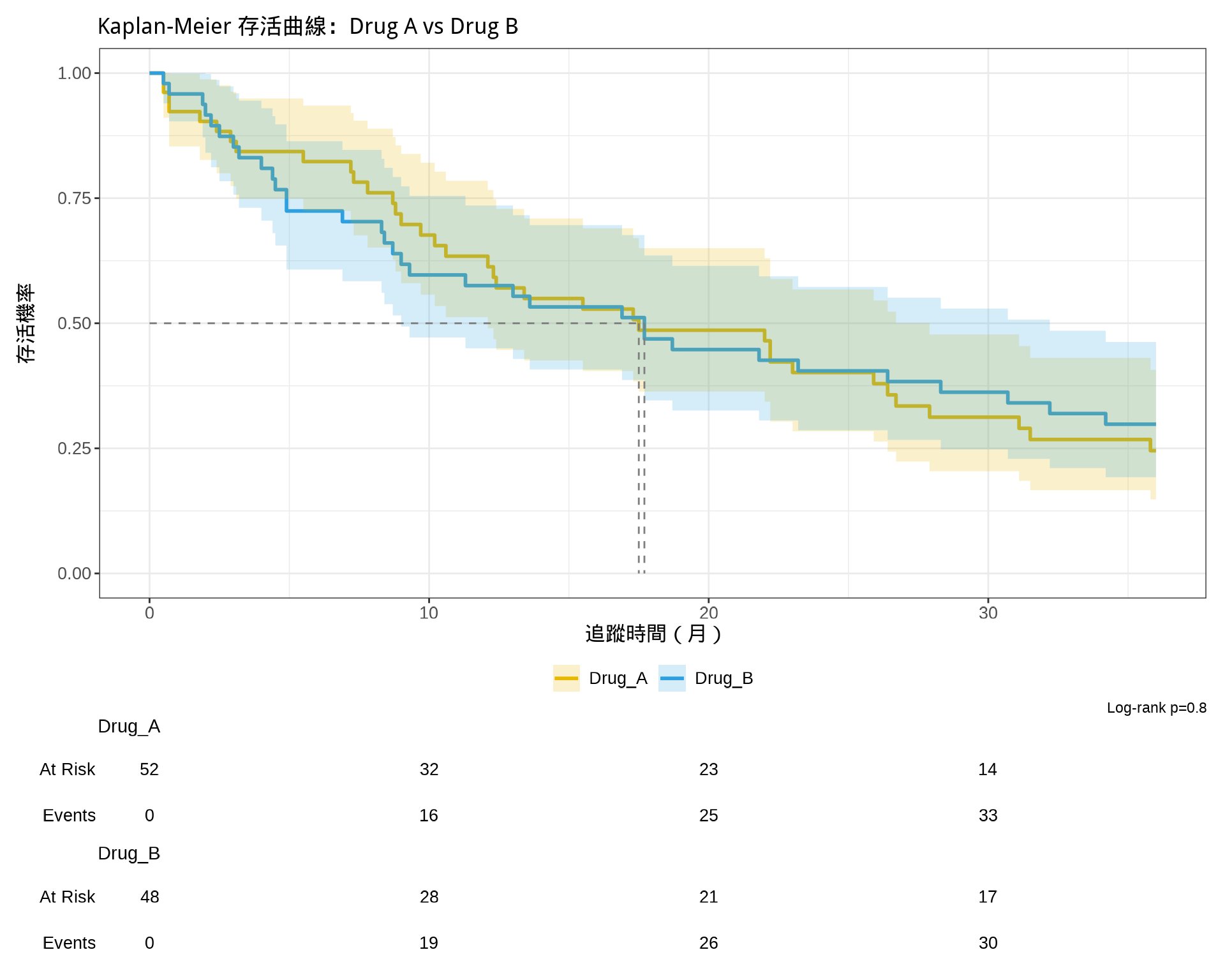
# 使用 ggsurvfit 繪製存活曲線(字型已由 _common.R 全域設定)
# survfit2() 是 ggsurvfit 的專用函數,可以更好地追蹤變數名稱
survfit2(Surv(time, status) ~ treatment, data = survival_data) |>
  ggsurvfit(linewidth = 1) +
  add_confidence_interval() +
  add_risktable() +
  add_pvalue(caption = "Log-rank {p.value}") +
  add_quantile(y_value = 0.5, linetype = "dashed", color = "gray50") +
  scale_color_manual(values = c("#E7B800", "#2E9FDF")) +
  scale_fill_manual(values = c("#E7B800", "#2E9FDF")) +
  labs(
    x = "追蹤時間(月)",
    y = "存活機率",
    title = "Kaplan-Meier 存活曲線:Drug A vs Drug B"
  ) +
  theme(legend.position = "bottom")
```
### 查看存活率摘要
```{r}
#| label: survival-summary
#| echo: true
# 依照治療組別做 Kaplan-Meier 分析
km_fit <- survfit(Surv(time, status) ~ treatment, data = survival_data)

# 查看摘要(6個月、12個月、24個月的存活率)
summary(km_fit, times = c(6, 12, 24))
```
### Log-Rank Test:比較兩組存活率
```{r}
#| label: survival-logrank
#| echo: true
# Log-rank test(最常用的存活曲線比較方法)
logrank_test <- survdiff(Surv(time, status) ~ treatment, data = survival_data)
print(logrank_test)
# 提取 p-value
logrank_pvalue <- 1 - pchisq(logrank_test$chisq, length(logrank_test$n) - 1)
print(paste("Log-rank test p-value:", round(logrank_pvalue, 4)))
# 解讀結果
if (logrank_pvalue < 0.05) {
  print("結論:兩組的存活曲線有顯著差異 (p < 0.05)")
} else {
  print("結論:兩組的存活曲線無顯著差異 (p >= 0.05)")
}
```
### 計算中位存活時間
```{r}
#| label: survival-median
#| echo: true
# 計算各組的中位存活時間
print("各組中位存活時間(月):")
print(km_fit)
# 使用 ggsurvfit 的 tidy 方式呈現
survfit2(Surv(time, status) ~ treatment, data = survival_data) |>
  tidy_survfit() |>
  head(10)
```
### 進階:Cox 比例風險模型
📋 **複製這段話,貼給 AI:**
> 我想要做更進階的存活分析,考慮多個變數(治療、年齡、性別、期別)對存活的影響。請幫我用 Cox proportional hazards model 分析,並解釋 Hazard Ratio 的意義。
```{r}
#| label: survival-cox
#| echo: true
#| message: false
# Cox 比例風險模型
# 可以同時考慮多個變數對存活的影響
cox_model <- coxph(
  Surv(time, status) ~ treatment + age + gender + stage,
  data = survival_data
)

# 查看模型結果
summary(cox_model)
# 整理成漂亮的表格
if (!require(gtsummary, quietly = TRUE)) {
  install.packages("gtsummary", repos = "https://cloud.r-project.org/")
}
library(gtsummary)

cox_model %>%
  tbl_regression(
    exponentiate = TRUE,  # 將係數轉換為 Hazard Ratio
    label = list(
      treatment ~ "治療組別",
      age ~ "年齡",
      gender ~ "性別",
      stage ~ "癌症期別"
    )
  ) %>%
  bold_p(t = 0.05) %>%
  modify_header(label = "**變數**") %>%
  modify_caption("**Cox 比例風險模型結果**")
```
### 存活分析結果解讀
```{r}
#| label: survival-interpretation
#| echo: true
# 提取 Hazard Ratio 和信賴區間
cox_summary <- summary(cox_model)
hr <- exp(cox_summary$coefficients[, "coef"])
ci_lower <- exp(cox_summary$coefficients[, "coef"] - 1.96 * cox_summary$coefficients[, "se(coef)"])
ci_upper <- exp(cox_summary$coefficients[, "coef"] + 1.96 * cox_summary$coefficients[, "se(coef)"])

# 整理成表格
hr_table <- data.frame(
  Variable = names(hr),
  HR = round(hr, 2),
  CI_Lower = round(ci_lower, 2),
  CI_Upper = round(ci_upper, 2),
  p_value = round(cox_summary$coefficients[, "Pr(>|z|)"], 4)
)
print(hr_table)
cat("\n=== Hazard Ratio 解讀指南 ===\n")
cat("HR = 1:該因素對存活沒有影響\n")
cat("HR > 1:該因素會增加死亡風險(例如 HR=2 表示風險增加一倍)\n")
cat("HR < 1:該因素會降低死亡風險(例如 HR=0.5 表示風險減半)\n")
```
### 小結:存活分析的關鍵概念
| 概念 | 說明 |
|------|------|
| **Censoring(設限)** | 觀察結束時事件尚未發生(例如病人還活著) |
| **Kaplan-Meier** | 估計存活機率隨時間變化的曲線 |
| **Log-rank test** | 比較兩組或多組存活曲線是否有差異 |
| **Hazard Ratio (HR)** | 相對風險,HR=2 表示風險是對照組的 2 倍 |
| **Cox model** | 可同時考慮多個變數對存活的影響 |