Code
flowchart LR
    A[概念理解] --> B[網絡幾何]
    B --> C[NMA 執行]
    C --> D[一致性評估]
    D --> E[排名分析]
    E --> F[學術報告]
flowchart LR
A[概念理解] --> B[網絡幾何]
B --> C[NMA 執行]
C --> D[一致性評估]
D --> E[排名分析]
E --> F[學術報告]
Network Meta-analysis with R
flowchart LR
    A[概念理解] --> B[網絡幾何]
    B --> C[NMA 執行]
    C --> D[一致性評估]
    D --> E[排名分析]
E --> F[學術報告]flowchart LR
A[概念理解] --> B[網絡幾何]
B --> C[NMA 執行]
C --> D[一致性評估]
D --> E[排名分析]
E --> F[學術報告]
研究問題:比較四種降血壓藥物(A、B、C、D)對收縮壓的相對效果
set.seed(2024)

# 網絡統合分析資料:比較四種降血壓藥物
nma_data <- data.frame(
  study = c("Wang 2018", "Chen 2019", "Liu 2020", "Zhang 2020",
            "Kim 2021", "Tanaka 2021", "Smith 2022", "Johnson 2023",
            "Lee 2019", "Park 2020", "Brown 2021", "Davis 2022"),
  treat1 = c("A", "A", "A", "B", "B", "C", "A", "B", "A", "C", "B", "C"),
  treat2 = c("B", "C", "D", "C", "D", "D", "B", "C", "C", "D", "D", "D"),
  n1 = c(45, 68, 52, 120, 38, 85, 63, 95, 55, 72, 48, 90),
  n2 = c(43, 65, 50, 118, 40, 82, 60, 92, 53, 70, 50, 88),
  mean1 = c(-12.3, -10.5, -14.2, -8.5, -9.2, -7.8, -11.8, -8.2, -10.8, -7.5, -9.0, -7.2),
  sd1 = c(8.2, 7.5, 9.1, 7.8, 7.2, 8.5, 7.9, 8.3, 7.6, 8.1, 7.4, 8.0),
  mean2 = c(-3.2, -4.5, -5.1, -4.8, -5.5, -4.2, -3.8, -4.5, -4.2, -3.8, -5.2, -3.5),
  sd2 = c(7.8, 7.2, 8.5, 7.5, 6.9, 8.1, 7.5, 7.9, 7.3, 7.8, 7.0, 7.6)
)knitr::kable(nma_data[, 1:5], caption = "研究基本資料")| study | treat1 | treat2 | n1 | n2 |
|---|---|---|---|---|
| Wang 2018 | A | B | 45 | 43 |
| Chen 2019 | A | C | 68 | 65 |
| Liu 2020 | A | D | 52 | 50 |
| Zhang 2020 | B | C | 120 | 118 |
| Kim 2021 | B | D | 38 | 40 |
| Tanaka 2021 | C | D | 85 | 82 |
| Smith 2022 | A | B | 63 | 60 |
| Johnson 2023 | B | C | 95 | 92 |
| Lee 2019 | A | C | 55 | 53 |
| Park 2020 | C | D | 72 | 70 |
| Brown 2021 | B | D | 48 | 50 |
| Davis 2022 | C | D | 90 | 88 |
| 欄位 | 說明 |
|---|---|
study |
研究名稱 |
treat1, treat2 |
比較的兩種治療 |
n1, n2 |
各組樣本數 |
mean1, mean2 |
各組平均值 |
sd1, sd2 |
各組標準差 |
# 計算每個比較的研究數
comparisons <- table(paste(nma_data$treat1, "vs", nma_data$treat2))
knitr::kable(as.data.frame(comparisons),
             col.names = c("比較", "研究數"),
caption = "各比較的研究數")| 比較 | 研究數 |
|---|---|
| A vs B | 2 |
| A vs C | 2 |
| A vs D | 1 |
| B vs C | 2 |
| B vs D | 2 |
| C vs D | 3 |
傳統統合分析像是「一對一比賽」,網絡統合分析像是「循環賽」——可以綜合所有選手的對戰結果,得出完整的排名。
傳統統合分析的限制
網絡統合分析的優勢
flowchart TD
    A[藥物 A] <-->|直接比較| B[藥物 B]
    A <-->|直接比較| C[藥物 C]
    B <-.->|間接比較| C
flowchart TD
A[藥物 A] <-->|直接比較| B[藥物 B]
A <-->|直接比較| C[藥物 C]
B <-.->|間接比較| C
| 證據類型 | 定義 | 來源 |
|---|---|---|
| 直接證據 | 兩種治療在同一研究中直接比較 | head-to-head RCT |
| 間接證據 | 透過共同比較組推論 | A vs B + A vs C → B vs C |
| 混合證據 | 直接與間接證據的結合 | 網絡統合分析 |
網絡統合分析假設直接與間接證據一致——這是有效性的基石
library(netmeta)
library(meta)
library(dplyr)# 計算標準化平均差
nma_data <- nma_data %>%
mutate(
# 計算 pooled SD
sd_pooled = sqrt(((n1-1)*sd1^2 + (n2-1)*sd2^2) / (n1 + n2 - 2)),
# 計算 SMD (Hedges' g)
smd = (mean1 - mean2) / sd_pooled,
# 計算 SE
se = sqrt((n1 + n2)/(n1 * n2) + smd^2/(2*(n1 + n2)))
)nma_result <- netmeta(
TE = smd,
seTE = se,
treat1 = treat1,
treat2 = treat2,
studlab = study,
data = nma_data,
sm = "SMD",
reference.group = "A",
common = FALSE,
random = TRUE
)netgraph(nma_result,
plastic = FALSE,
thickness = "number.of.studies",
points = TRUE,
cex.points = 3,
col = "steelblue",
multiarm = TRUE,
number.of.studies = TRUE)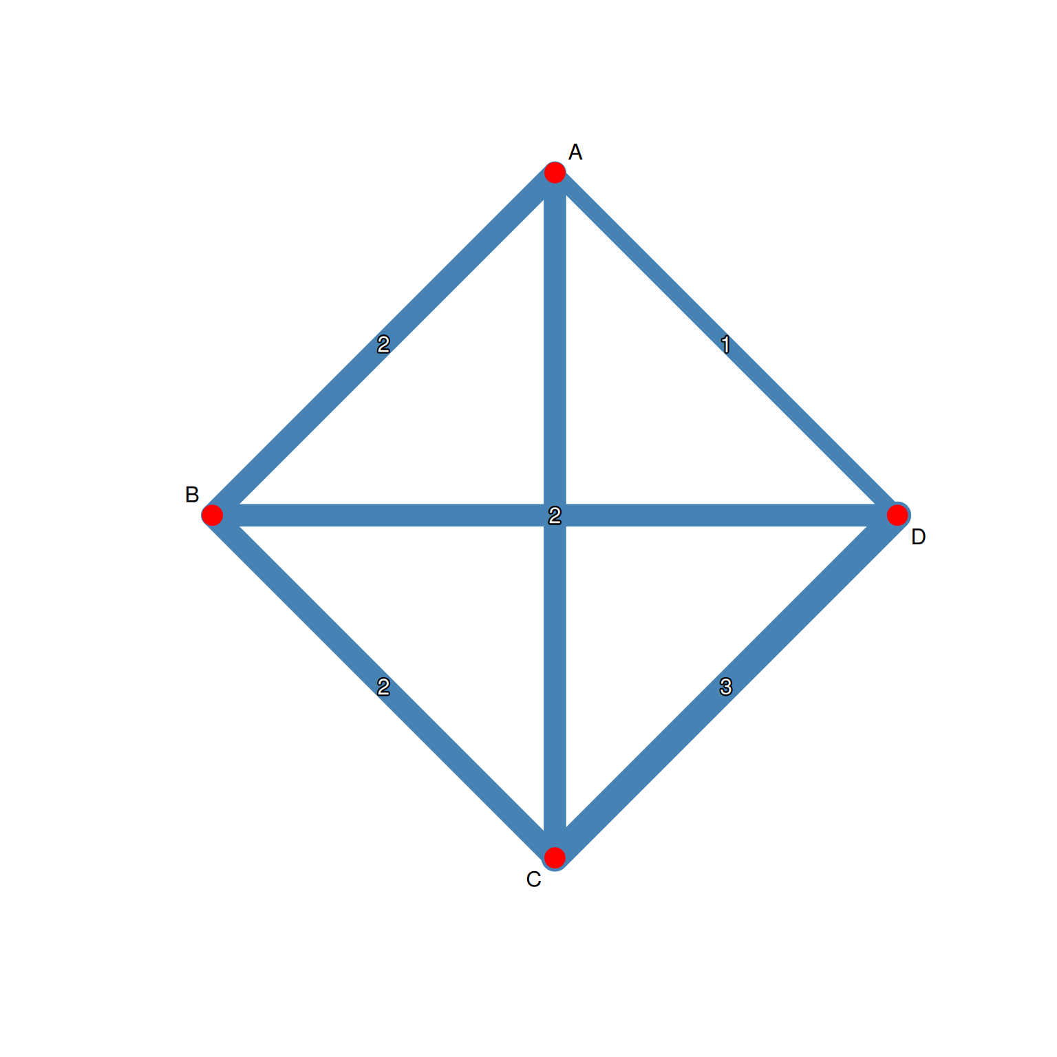
| 元素 | 意義 |
|---|---|
| 節點 | 治療選項 |
| 節點大小 | 該治療的總樣本數 |
| 連線 | 存在直接比較 |
| 連線粗細 | 研究數量 |
# 檢視網絡基本資訊
cat("治療數:", nma_result$n, "\n")
治療數: 4 cat("研究數:", nma_result$k, "\n")研究數: 12 cat("比較數:", nma_result$m, "\n")比較數: 12 summary(nma_result)Original data:
treat1 treat2 TE seTE
Wang 2018 A B -1.1365 0.2298
Chen 2019 A C -0.8158 0.1805
Liu 2020 A D -1.0328 0.2109
Zhang 2020 B C -0.4835 0.1315
Kim 2021 B D -0.5250 0.2304
Tanaka 2021 C D -0.4334 0.1566
Smith 2022 A B -1.0379 0.1921
Johnson 2023 B C -0.4565 0.1482
Lee 2019 A C -0.8854 0.2017
Park 2020 C D -0.4652 0.1701
Brown 2021 B D -0.5279 0.2056
Davis 2022 C D -0.4741 0.1520
Number of treatment arms per study:
narms
Wang 2018 2
Chen 2019 2
Liu 2020 2
Zhang 2020 2
Kim 2021 2
Tanaka 2021 2
Smith 2022 2
Johnson 2023 2
Lee 2019 2
Park 2020 2
Brown 2021 2
Davis 2022 2
Results (random effects model):
treat1 treat2 SMD 95%-CI
Wang 2018 A B -0.7609 [-1.0133; -0.5085]
Chen 2019 A C -0.9934 [-1.2354; -0.7514]
Liu 2020 A D -1.3482 [-1.6185; -1.0779]
Zhang 2020 B C -0.2325 [-0.4460; -0.0190]
Kim 2021 B D -0.5873 [-0.8264; -0.3481]
Tanaka 2021 C D -0.3548 [-0.5594; -0.1502]
Smith 2022 A B -0.7609 [-1.0133; -0.5085]
Johnson 2023 B C -0.2325 [-0.4460; -0.0190]
Lee 2019 A C -0.9934 [-1.2354; -0.7514]
Park 2020 C D -0.3548 [-0.5594; -0.1502]
Brown 2021 B D -0.5873 [-0.8264; -0.3481]
Davis 2022 C D -0.3548 [-0.5594; -0.1502]
Number of studies: k = 12
Number of pairwise comparisons: m = 12
Number of treatments: n = 4
Number of designs: d = 6
Random effects model
Treatment estimate (other treatments vs 'A'):
SMD 95%-CI z p-value
A . . . .
B 0.7609 [0.5085; 1.0133] 5.91 < 0.0001
C 0.9934 [0.7514; 1.2354] 8.05 < 0.0001
D 1.3482 [1.0779; 1.6185] 9.78 < 0.0001
Quantifying heterogeneity / inconsistency:
tau^2 = 0.0221; tau = 0.1485; I^2 = 41.2% [0.0%; 71.9%]
Tests of heterogeneity (within designs) and inconsistency (between designs):
Q d.f. p-value
Total 15.31 9 0.0829
Within designs 0.23 6 0.9998
Between designs 15.07 3 0.0018
Details of network meta-analysis methods:
- Frequentist graph-theoretical approach
- DerSimonian-Laird estimator for tau^2
- Calculation of I^2 based on Qnetleague <- netleague(nma_result,
bracket = "(",
digits = 2)
print(netleague)League table (random effects model):
A -1.08 (-1.44; -0.73) -0.85 (-1.18; -0.51)
-0.76 (-1.01; -0.51) B -0.47 (-0.75; -0.19)
-0.99 (-1.24; -0.75) -0.23 (-0.45; -0.02) C
-1.35 (-1.62; -1.08) -0.59 (-0.83; -0.35) -0.35 (-0.56; -0.15)
-1.03 (-1.54; -0.53)
-0.53 (-0.89; -0.16)
-0.46 (-0.70; -0.21)
D
Lower triangle: results from network meta-analysis (column vs row)
Upper triangle: results from direct comparisons (row vs column)forest(nma_result,
reference.group = "A",
sortvar = TE,
smlab = "SMD vs. Treatment A",
drop.reference.group = TRUE,
label.left = "Favors treatment",
label.right = "Favors A")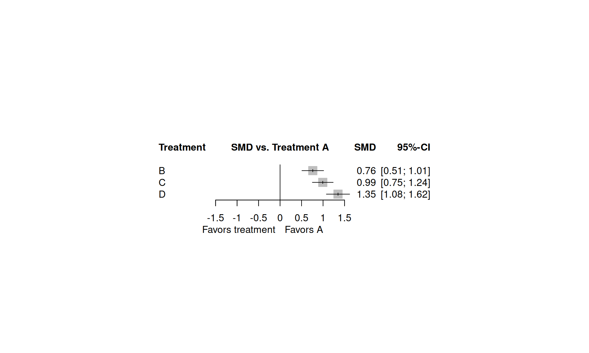
This network meta-analysis included 12 RCTs comparing 4 treatments (A, B, C, D). Using treatment A as the reference, the random-effects model showed that all treatments significantly reduced blood pressure compared to A. Treatment D showed the largest effect (SMD = −XX, 95% CI: −XX to −XX).
# Q 統計量分解
decomp <- decomp.design(nma_result)
print(decomp)
Q statistics to assess homogeneity / consistency
Q df p-value
Total 15.31 9 0.0829
Within designs 0.23 6 0.9998
Between designs 15.07 3 0.0018
Design-specific decomposition of within-designs Q statistic
Design Q df p-value
A:B 0.11 1 0.7422
A:C 0.07 1 0.7970
B:C 0.02 1 0.8915
C:D 0.04 2 0.9814
B:D 0.00 1 0.9926
Between-designs Q statistic after detaching of single designs
(influential designs have p-value markedly different from 0.0018)
Detached design Q df p-value
B:C 3.65 2 0.1609
A:B 4.41 2 0.1101
C:D 10.86 2 0.0044
A:D 11.76 2 0.0028
A:C 12.26 2 0.0022
B:D 14.33 2 0.0008
Q statistic to assess consistency under the assumption of
a full design-by-treatment interaction random effects model
Q df p-value tau.within tau2.within
Between designs 15.07 3 0.0018 0 0# 節點分割法
netsplit_result <- netsplit(nma_result)
print(netsplit_result)Separate indirect from direct evidence (SIDE) using back-calculation method
Random effects model:
comparison k prop nma direct indir. Diff z p-value
B:A 2 0.50 0.7609 1.0814 0.4371 0.6443 2.50 0.0124
C:A 2 0.52 0.9934 0.8482 1.1519 -0.3037 -1.23 0.2191
D:A 1 0.29 1.3482 1.0328 1.4745 -0.4417 -1.45 0.1478
B:C 2 0.57 -0.2325 -0.4707 0.0847 -0.5554 -2.52 0.0116
B:D 2 0.43 -0.5873 -0.5266 -0.6331 0.1065 0.43 0.6657
C:D 3 0.69 -0.3548 -0.4575 -0.1274 -0.3301 -1.46 0.1431
Legend:
comparison - Treatment comparison
k - Number of studies providing direct evidence
prop - Direct evidence proportion
nma - Estimated treatment effect (SMD) in network meta-analysis
direct - Estimated treatment effect (SMD) derived from direct evidence
indir. - Estimated treatment effect (SMD) derived from indirect evidence
Diff - Difference between direct and indirect treatment estimates
z - z-value of test for disagreement (direct versus indirect)
p-value - p-value of test for disagreement (direct versus indirect)forest(netsplit_result,
show = "both",
fontsize = 8)
| 指標 | 閾值 | 解讀 |
|---|---|---|
| Q (設計間) | p < 0.10 | 存在設計間不一致性 |
| 節點分割 p 值 | p < 0.10 | 該比較存在不一致性 |
| RoR (Ratio of Ratios) | 顯著偏離 1 | 直接與間接證據不一致 |
cat("Tau²:", round(nma_result$tau^2, 4), "\n")Tau²: 0.0221 cat("I² (within-design):", round(nma_result$I2, 1), "%\n")I² (within-design): 0.4 %# 按比較分組的異質性
het_data <- data.frame(
Comparison = paste(nma_data$treat1, "vs", nma_data$treat2),
SMD = round(nma_data$smd, 2),
Study = nma_data$study
)
knitr::kable(het_data, caption = "各研究效果量")| Comparison | SMD | Study |
|---|---|---|
| A vs B | -1.14 | Wang 2018 |
| A vs C | -0.82 | Chen 2019 |
| A vs D | -1.03 | Liu 2020 |
| B vs C | -0.48 | Zhang 2020 |
| B vs D | -0.52 | Kim 2021 |
| C vs D | -0.43 | Tanaka 2021 |
| A vs B | -1.04 | Smith 2022 |
| B vs C | -0.46 | Johnson 2023 |
| A vs C | -0.89 | Lee 2019 |
| C vs D | -0.47 | Park 2020 |
| B vs D | -0.53 | Brown 2021 |
| C vs D | -0.47 | Davis 2022 |
# 計算 P-score
ranking <- netrank(nma_result, small.values = "desirable")
print(ranking)
P-score
A 1.0000
B 0.6612
C 0.3387
D 0.0001# 繪製 rankogram
plot(ranking)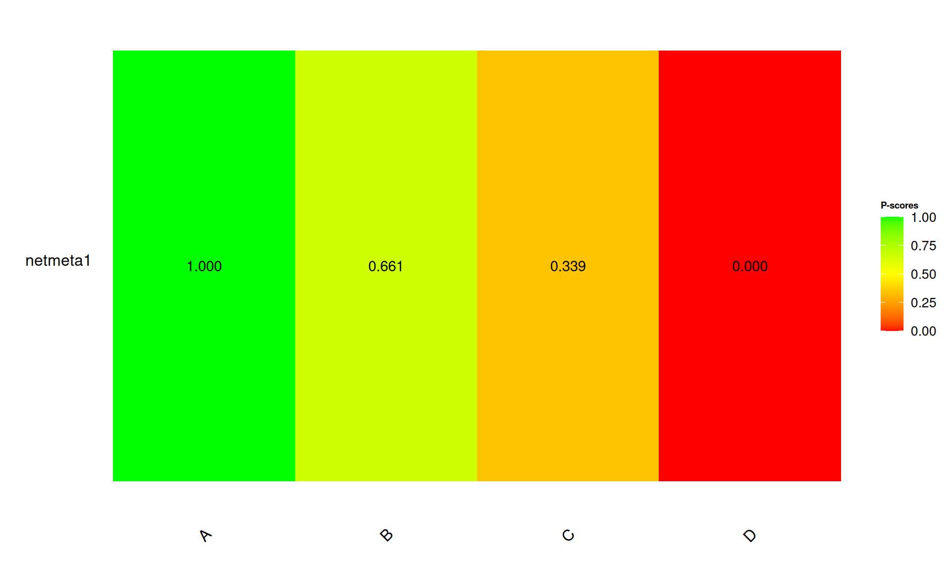
| P-score / SUCRA | 解讀 |
|---|---|
| > 80% | 很可能是最佳治療 |
| 50-80% | 中等排名 |
| < 50% | 較差排名 |
# 建立排名摘要表
rank_summary <- data.frame(
  Treatment = names(ranking$Pscore.random),
  P_score = round(ranking$Pscore.random, 3)
)
rank_summary <- rank_summary[order(-rank_summary$P_score), ]
rownames(rank_summary) <- NULL
knitr::kable(rank_summary, caption = "治療排名摘要")| Treatment | P_score |
|---|---|
| A | 1.000 |
| B | 0.661 |
| C | 0.339 |
| D | 0.000 |
# 新增年份分組
nma_data$period <- ifelse(
  as.numeric(gsub(".*?(\\d{4}).*", "\\1", nma_data$study)) < 2021,
  "2018-2020",
  "2021-2023"
)

# 分組執行 NMA
table(nma_data$period)
2018-2020 2021-2023
6 6 # 以樣本數為協變數
nma_data$total_n <- nma_data$n1 + nma_data$n2
# 執行網絡統合迴歸(示例)
# 注意:netmetareg 需要足夠的研究數
cat("平均樣本數:", round(mean(nma_data$total_n), 1), "\n")平均樣本數: 136.8 cat("樣本數範圍:", min(nma_data$total_n), "-", max(nma_data$total_n), "\n")樣本數範圍: 78 - 238 funnel(nma_result,
order = c("A", "B", "C", "D"),
legend = TRUE)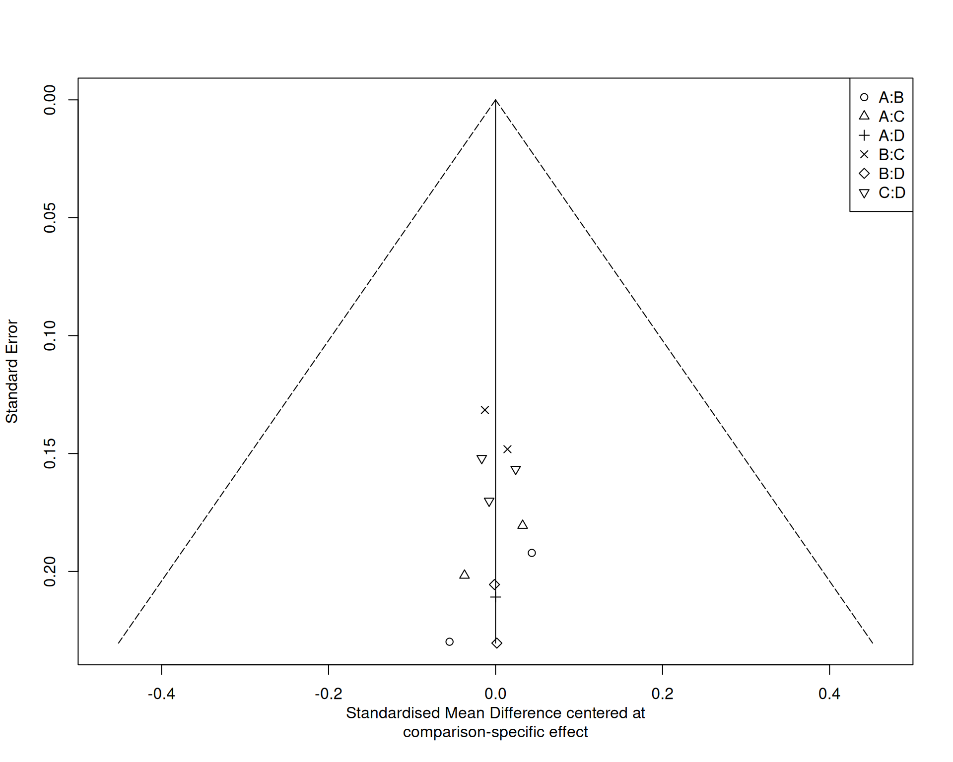
Visual inspection of the comparison-adjusted funnel plot did not reveal obvious asymmetry. However, given the limited number of studies per comparison, formal testing for publication bias was not performed.
# 逐一排除研究
loo_results <- list()
for(i in 1:nrow(nma_data)) {
  temp_data <- nma_data[-i, ]
  temp_nma <- netmeta(
    TE = smd,
    seTE = se,
    treat1 = treat1,
    treat2 = treat2,
    studlab = study,
    data = temp_data,
    sm = "SMD",
    reference.group = "A",
    random = TRUE,
    common = FALSE
  )
  loo_results[[nma_data$study[i]]] <- temp_nma$TE.random
}# 比較各治療相對於 A 的效果穩定性
cat("原始分析 B vs A:", round(nma_result$TE.random["B", "A"], 3), "\n")原始分析 B vs A: 0.761 cat("原始分析 C vs A:", round(nma_result$TE.random["C", "A"], 3), "\n")原始分析 C vs A: 0.993 cat("原始分析 D vs A:", round(nma_result$TE.random["D", "A"], 3), "\n")原始分析 D vs A: 1.348 # 比較固定效應與隨機效應模型
nma_fixed <- netmeta(
TE = smd,
seTE = se,
treat1 = treat1,
treat2 = treat2,
studlab = study,
data = nma_data,
sm = "SMD",
reference.group = "A",
common = TRUE,
random = FALSE
)
comparison_df <- data.frame(
Comparison = c("B vs A", "C vs A", "D vs A"),
Random = round(c(nma_result$TE.random["B", "A"],
nma_result$TE.random["C", "A"],
nma_result$TE.random["D", "A"]), 3),
Fixed = round(c(nma_fixed$TE.common["B", "A"],
nma_fixed$TE.common["C", "A"],
nma_fixed$TE.common["D", "A"]), 3)
)
knitr::kable(comparison_df, caption = "模型比較")| Comparison | Random | Fixed |
|---|---|---|
| B vs A | 0.761 | 0.730 |
| C vs A | 0.993 | 1.003 |
| D vs A | 1.348 | 1.361 |
必要項目
進階項目
summary_df <- data.frame(
  指標 = c("納入研究數", "治療選項數", "總樣本數",
           "最佳治療", "P-score", "I²"),
  數值 = c(nma_result$k,
           nma_result$n,
           sum(nma_data$n1) + sum(nma_data$n2),
           rank_summary$Treatment[1],
           paste0(rank_summary$P_score[1] * 100, "%"),
           paste0(round(nma_result$I2, 1), "%"))
)
knitr::kable(summary_df, caption = "網絡統合分析結果摘要")| 指標 | 數值 |
|---|---|
| 納入研究數 | 12 |
| 治療選項數 | 4 |
| 總樣本數 | 1642 |
| 最佳治療 | A |
| P-score | 100% |
| I² | 0.4% |
This network meta-analysis included 12 RCTs comparing 4 treatments. The network was well-connected with all treatments having at least one direct comparison. Using the random-effects model, Treatment A showed the highest probability of being the best treatment (P-score = 1). No significant inconsistency was detected between direct and indirect evidence. The results remained robust in sensitivity analyses.
| 比較 | 證據品質 | 降級原因 |
|---|---|---|
| D vs A | 中等 | 間接性 |
| C vs A | 中等 | 間接性 |
| B vs A | 高 | - |
| 項目 | 完成 |
|---|---|
| 明確定義研究問題 (PICO) | ☐ |
| 事先註冊 (PROSPERO) | ☐ |
| 制定納入/排除標準 | ☐ |
| 確認網絡可連通 | ☐ |
| 項目 | 完成 |
|---|---|
| 繪製網絡幾何圖 | ☐ |
| 選擇適當效果量 | ☐ |
| 執行網絡統合分析 | ☐ |
| 評估一致性 | ☐ |
| 評估異質性 | ☐ |
| 計算治療排名 | ☐ |
| 發表偏誤評估 | ☐ |
| 敏感度分析 | ☐ |
| 項目 | 完成 |
|---|---|
| 遵循 PRISMA-NMA 指引 | ☐ |
| 呈現 League table | ☐ |
| 報告一致性結果 | ☐ |
| GRADE 評估證據品質 | ☐ |
| 面向 | 傳統統合分析 | 網絡統合分析 |
|---|---|---|
| 比較數 | 2 種治療 | ≥ 3 種治療 |
| 證據類型 | 僅直接 | 直接 + 間接 |
| 排名 | 無 | 有 |
| 一致性 | 不適用 | 需評估 |
| 複雜度 | 較低 | 較高 |
資料格式要求:
study,treat1,treat2,n1,n2,mean1,sd1,mean2,sd2
Author1 2020,A,B,50,48,10.2,3.5,8.1,3.2
Author2 2021,B,C,75,72,11.5,4.1,9.2,3.8
Author3 2021,A,C,60,58,10.8,3.8,8.5,3.5有任何問題歡迎討論