flowchart LR
    A[概念理解] --> B[網絡幾何]
    B --> C[NMA 執行]
    C --> D[一致性評估]
    D --> E[排名分析]
    E --> F[學術報告]
AI 輔助網絡統合分析教學
Network Meta-analysis with R
醫學統計教學課程
2025-12-10
課程簡介
學習目標
- 理解網絡統合分析的基本概念
- 學會使用 R 進行網絡統合分析
- 掌握結果解讀與學術寫作
- 培養批判性思維
課程架構
模擬情境
研究問題:比較四種降血壓藥物(A、B、C、D)對收縮壓的相對效果
- 12 篇 RCT 研究
- 涉及多組直接與間接比較
- 網絡統合分析
模擬資料
建立資料
Code
set.seed(2024)

nma_data <- data.frame(
  study = c("Wang 2018", "Chen 2019", "Liu 2020", "Zhang 2020",
            "Kim 2021", "Tanaka 2021", "Smith 2022", "Johnson 2023",
            "Lee 2019", "Park 2020", "Brown 2021", "Davis 2022"),
  treat1 = c("A", "A", "A", "B", "B", "C", "A", "B", "A", "C", "B", "C"),
  treat2 = c("B", "C", "D", "C", "D", "D", "B", "C", "C", "D", "D", "D"),
  n1 = c(45, 68, 52, 120, 38, 85, 63, 95, 55, 72, 48, 90),
  n2 = c(43, 65, 50, 118, 40, 82, 60, 92, 53, 70, 50, 88),
  mean1 = c(-12.3, -10.5, -14.2, -8.5, -9.2, -7.8, -11.8, -8.2, -10.8, -7.5, -9.0, -7.2),
  sd1 = c(8.2, 7.5, 9.1, 7.8, 7.2, 8.5, 7.9, 8.3, 7.6, 8.1, 7.4, 8.0),
  mean2 = c(-3.2, -4.5, -5.1, -4.8, -5.5, -4.2, -3.8, -4.5, -4.2, -3.8, -5.2, -3.5),
  sd2 = c(7.8, 7.2, 8.5, 7.5, 6.9, 8.1, 7.5, 7.9, 7.3, 7.8, 7.0, 7.6)
)
資料預覽
| study | treat1 | treat2 | n1 | n2 |
|---|---|---|---|---|
| Wang 2018 | A | B | 45 | 43 |
| Chen 2019 | A | C | 68 | 65 |
| Liu 2020 | A | D | 52 | 50 |
| Zhang 2020 | B | C | 120 | 118 |
| Kim 2021 | B | D | 38 | 40 |
| Tanaka 2021 | C | D | 85 | 82 |
| Smith 2022 | A | B | 63 | 60 |
| Johnson 2023 | B | C | 95 | 92 |
| Lee 2019 | A | C | 55 | 53 |
| Park 2020 | C | D | 72 | 70 |
| Brown 2021 | B | D | 48 | 50 |
| Davis 2022 | C | D | 90 | 88 |
資料結構
| 欄位 | 說明 |
|---|---|
study |
研究名稱 |
treat1, treat2 |
比較的兩種治療 |
n1, n2 |
各組樣本數 |
mean1, mean2 |
各組平均值 |
sd1, sd2 |
各組標準差 |
任務一:基本概念
什麼是網絡統合分析?
比喻
傳統統合分析像是「一對一比賽」,網絡統合分析像是「循環賽」
- 合併多種治療的直接與間接比較
- 同時比較三個以上的治療選項
- 產生完整的治療排名
為什麼需要網絡統合分析?
傳統統合分析的限制
- 只能比較兩種治療
- 無法整合間接證據
- 難以產生完整排名
網絡統合分析的優勢
- 同時比較多種治療
- 整合直接與間接證據
- 產生治療效果排名
直接與間接證據
一致性假設
核心假設
網絡統合分析假設直接與間接證據一致
- 若 A 優於 B,A 也優於 C
- 則間接推論 B 與 C 的關係應與直接比較一致
任務二:網絡幾何
載入套件
計算效果量
建立網絡物件
網絡圖
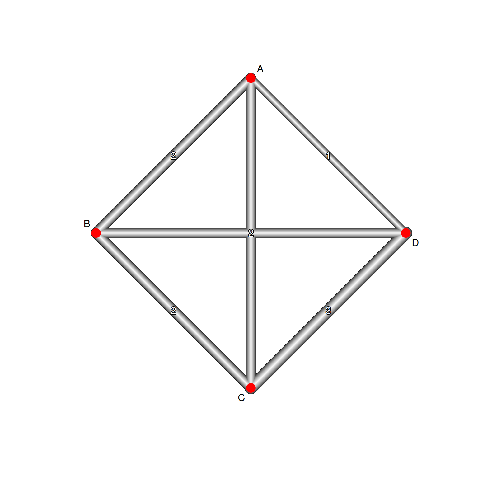
網絡幾何解讀
| 元素 | 意義 |
|---|---|
| 節點 | 治療選項 |
| 節點大小 | 該治療的總樣本數 |
| 連線 | 存在直接比較 |
| 連線粗細 | 研究數量 |
任務三:網絡統合分析
執行網絡統合分析
Original data:

             treat1 treat2      TE   seTE
Wang 2018         A      B -1.1365 0.2298
Chen 2019         A      C -0.8158 0.1805
Liu 2020          A      D -1.0328 0.2109
Zhang 2020        B      C -0.4835 0.1315
Kim 2021          B      D -0.5250 0.2304
Tanaka 2021       C      D -0.4334 0.1566
Smith 2022        A      B -1.0379 0.1921
Johnson 2023      B      C -0.4565 0.1482
Lee 2019          A      C -0.8854 0.2017
Park 2020         C      D -0.4652 0.1701
Brown 2021        B      D -0.5279 0.2056
Davis 2022        C      D -0.4741 0.1520

Number of treatment arms per study:
             narms
Wang 2018        2
Chen 2019        2
Liu 2020         2
Zhang 2020       2
Kim 2021         2
Tanaka 2021      2
Smith 2022       2
Johnson 2023     2
Lee 2019         2
Park 2020        2
Brown 2021       2
Davis 2022       2

Results (random effects model):

             treat1 treat2     SMD             95%-CI
Wang 2018         A      B -0.7609 [-1.0133; -0.5085]
Chen 2019         A      C -0.9934 [-1.2354; -0.7514]
Liu 2020          A      D -1.3482 [-1.6185; -1.0779]
Zhang 2020        B      C -0.2325 [-0.4460; -0.0190]
Kim 2021          B      D -0.5873 [-0.8264; -0.3481]
Tanaka 2021       C      D -0.3548 [-0.5594; -0.1502]
Smith 2022        A      B -0.7609 [-1.0133; -0.5085]
Johnson 2023      B      C -0.2325 [-0.4460; -0.0190]
Lee 2019          A      C -0.9934 [-1.2354; -0.7514]
Park 2020         C      D -0.3548 [-0.5594; -0.1502]
Brown 2021        B      D -0.5873 [-0.8264; -0.3481]
Davis 2022        C      D -0.3548 [-0.5594; -0.1502]

Number of studies: k = 12
Number of pairwise comparisons: m = 12
Number of treatments: n = 4
Number of designs: d = 6

Random effects model

Treatment estimate (other treatments vs 'A'):
     SMD           95%-CI    z  p-value
A      .                .    .        .
B 0.7609 [0.5085; 1.0133] 5.91 < 0.0001
C 0.9934 [0.7514; 1.2354] 8.05 < 0.0001
D 1.3482 [1.0779; 1.6185] 9.78 < 0.0001

Quantifying heterogeneity / inconsistency:
tau^2 = 0.0221; tau = 0.1485; I^2 = 41.2% [0.0%; 71.9%]

Tests of heterogeneity (within designs) and inconsistency (between designs):
                    Q d.f. p-value
Total           15.31    9  0.0829
Within designs   0.23    6  0.9998
Between designs 15.07    3  0.0018

Details of network meta-analysis methods:
- Frequentist graph-theoretical approach
- DerSimonian-Laird estimator for tau^2
- Calculation of I^2 based on Q
League Table
League table (random effects model):

                    A -1.08 (-1.44; -0.73) -0.85 (-1.18; -0.51)
 -0.76 (-1.01; -0.51)                    B -0.47 (-0.75; -0.19)
 -0.99 (-1.24; -0.75) -0.23 (-0.45; -0.02)                    C
 -1.35 (-1.62; -1.08) -0.59 (-0.83; -0.35) -0.35 (-0.56; -0.15)

 -1.03 (-1.54; -0.53)
 -0.53 (-0.89; -0.16)
 -0.46 (-0.70; -0.21)
                    D

Lower triangle: results from network meta-analysis (column vs row)
Upper triangle: results from direct comparisons (row vs column)
森林圖:相對於參照組
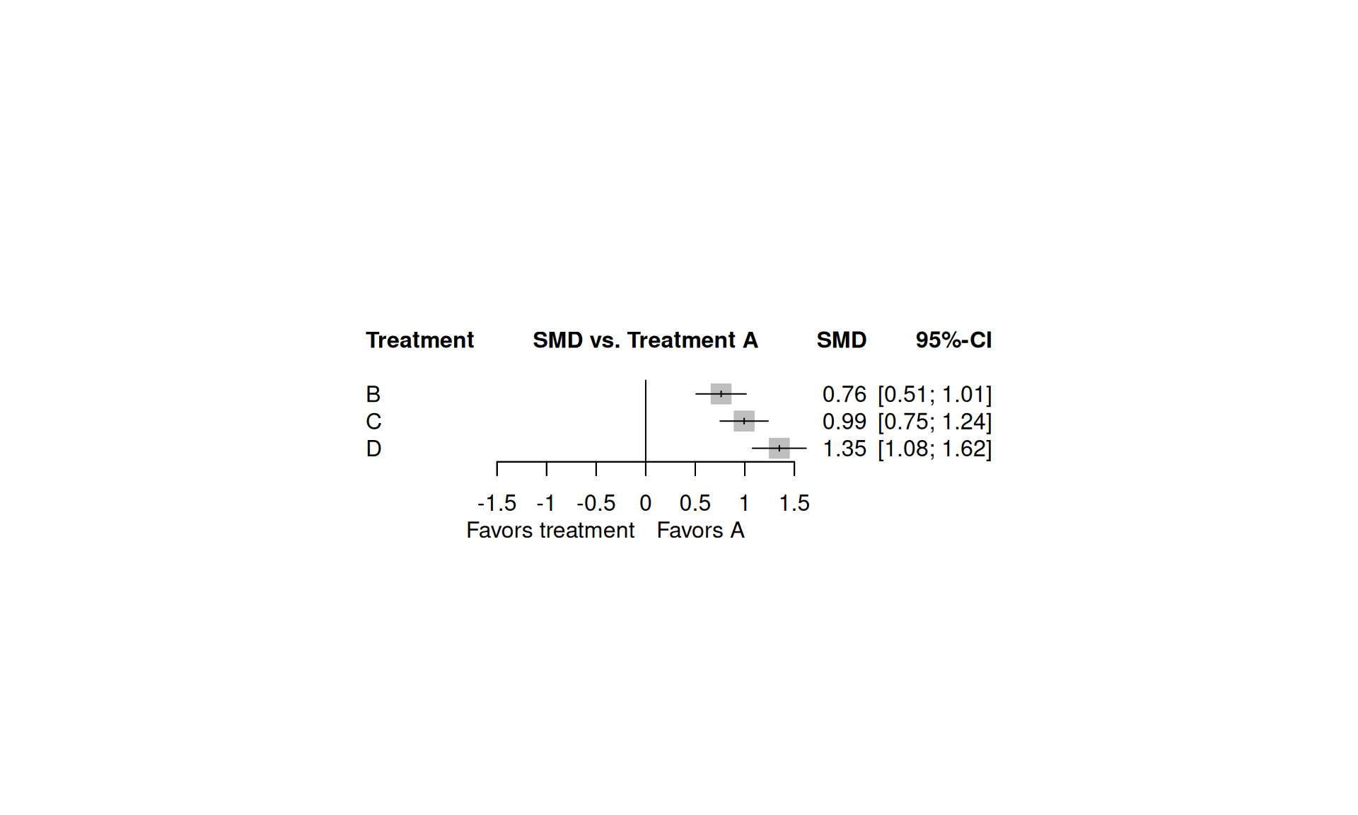
學術寫作範例
Results
This network meta-analysis included 12 RCTs comparing 4 treatments. Using treatment A as the reference, all treatments significantly reduced blood pressure.
任務四:一致性評估
為什麼要評估一致性?
- 確保直接與間接證據不矛盾
- 驗證網絡統合分析的有效性
- 識別潛在的異質性來源
全域一致性檢定
Q statistics to assess homogeneity / consistency
Q df p-value
Total 15.31 9 0.0829
Within designs 0.23 6 0.9998
Between designs 15.07 3 0.0018
Design-specific decomposition of within-designs Q statistic
Design Q df p-value
A:B 0.11 1 0.7422
A:C 0.07 1 0.7970
B:C 0.02 1 0.8915
C:D 0.04 2 0.9814
B:D 0.00 1 0.9926
Between-designs Q statistic after detaching of single designs
(influential designs have p-value markedly different from 0.0018)
Detached design Q df p-value
B:C 3.65 2 0.1609
A:B 4.41 2 0.1101
C:D 10.86 2 0.0044
A:D 11.76 2 0.0028
A:C 12.26 2 0.0022
B:D 14.33 2 0.0008
Q statistic to assess consistency under the assumption of
a full design-by-treatment interaction random effects model
Q df p-value tau.within tau2.within
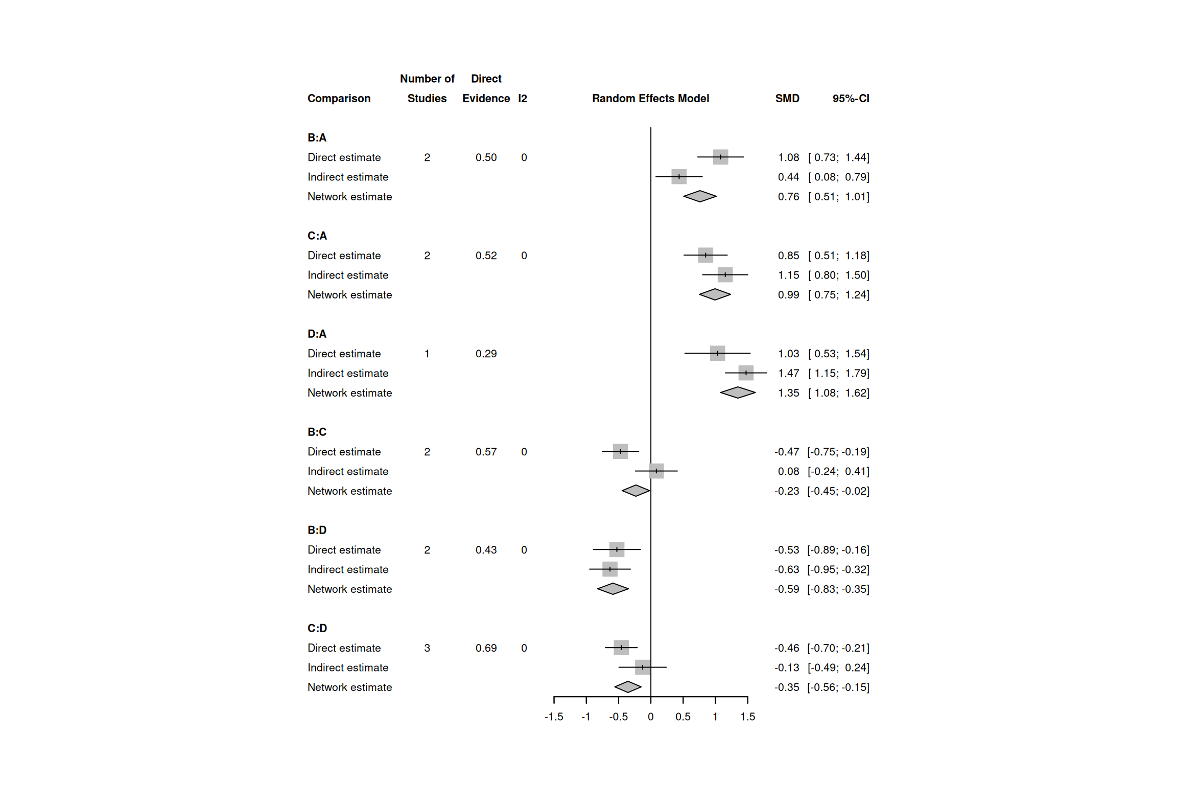
Between designs 15.07 3 0.0018 0 0局部一致性檢定
Separate indirect from direct evidence (SIDE) using back-calculation method

Random effects model:

 comparison k prop     nma  direct  indir.    Diff     z p-value
        B:A 2 0.50  0.7609  1.0814  0.4371  0.6443  2.50  0.0124
        C:A 2 0.52  0.9934  0.8482  1.1519 -0.3037 -1.23  0.2191
        D:A 1 0.29  1.3482  1.0328  1.4745 -0.4417 -1.45  0.1478
        B:C 2 0.57 -0.2325 -0.4707  0.0847 -0.5554 -2.52  0.0116
        B:D 2 0.43 -0.5873 -0.5266 -0.6331  0.1065  0.43  0.6657
        C:D 3 0.69 -0.3548 -0.4575 -0.1274 -0.3301 -1.46  0.1431

Legend:
 comparison - Treatment comparison
 k          - Number of studies providing direct evidence
 prop       - Direct evidence proportion
 nma        - Estimated treatment effect (SMD) in network meta-analysis
 direct     - Estimated treatment effect (SMD) derived from direct evidence
 indir.     - Estimated treatment effect (SMD) derived from indirect evidence
 Diff       - Difference between direct and indirect treatment estimates
 z          - z-value of test for disagreement (direct versus indirect)
 p-value    - p-value of test for disagreement (direct versus indirect)
一致性森林圖
一致性解讀標準
| 指標 | 閾值 | 解讀 |
|---|---|---|
| Q (設計間) | p < 0.10 | 存在設計間不一致性 |
| 節點分割 p 值 | p < 0.10 | 該比較存在不一致性 |
任務五:異質性評估
異質性指標
I² 解讀標準
| I² 值 | 異質性程度 |
|---|---|
| < 25% | 低度 |
| 25-50% | 中度 |
| 50-75% | 中高度 |
| > 75% | 高度 |
討論重點
- 網絡內異質性 vs. 設計間異質性
- τ² 的臨床意義
- 高異質性時如何解讀排名
任務六:排名分析
P-score 排名
排名圖
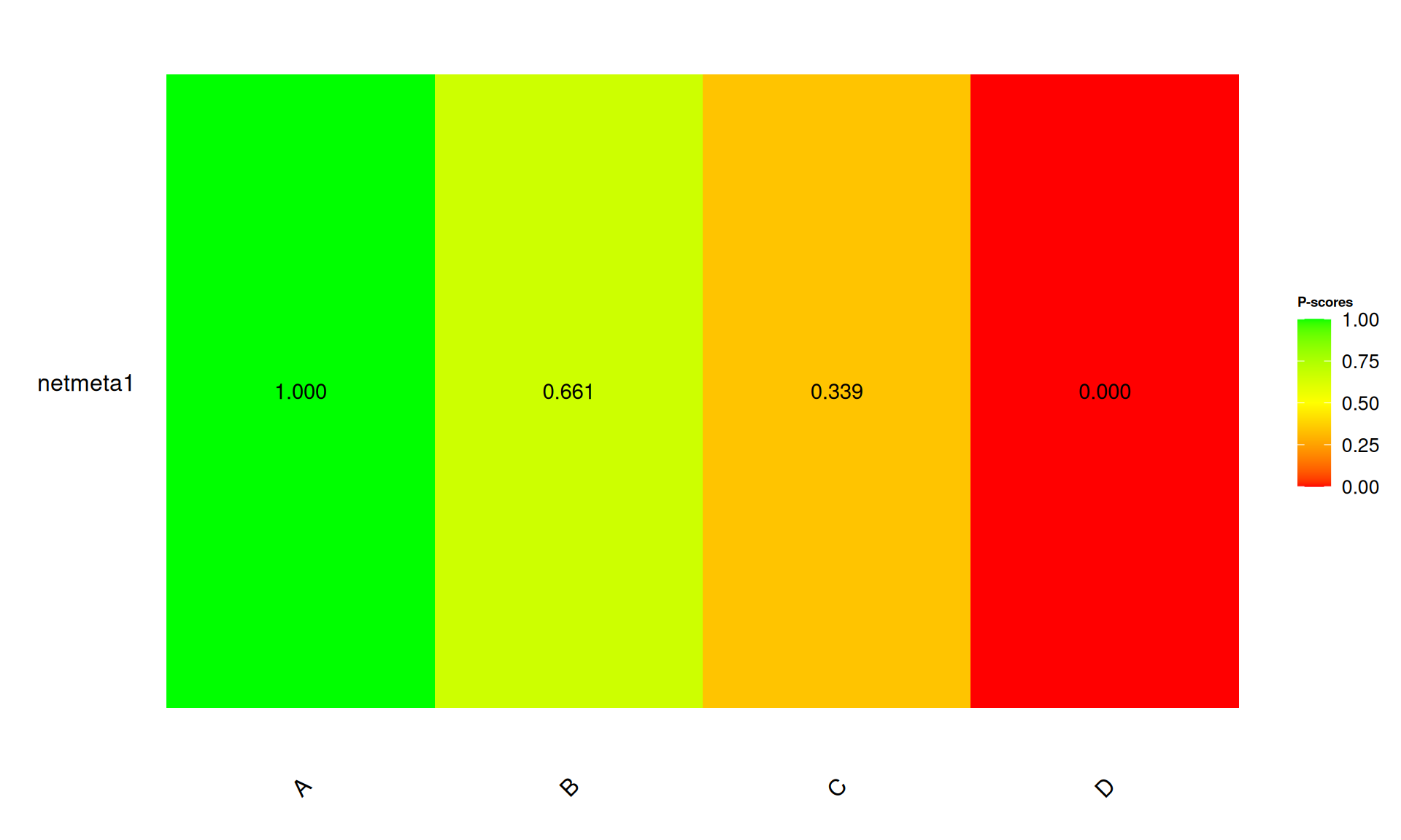
SUCRA 概念
Surface Under the Cumulative Ranking (SUCRA)
- 範圍:0% 到 100%
- 越高代表該治療排名越好的機率越高
排名的不確定性
謹慎解讀排名
- 排名差異可能不具統計顯著性
- 應同時考慮信賴區間
- 最佳治療不一定顯著優於第二名
任務七:次群體分析
次群體網絡統合分析
注意事項
網絡統合迴歸的限制
- 需要更多研究數
- 共變數需在網絡中有足夠變異
- 生態謬誤風險
任務八:發表偏誤
比較校正漏斗圖
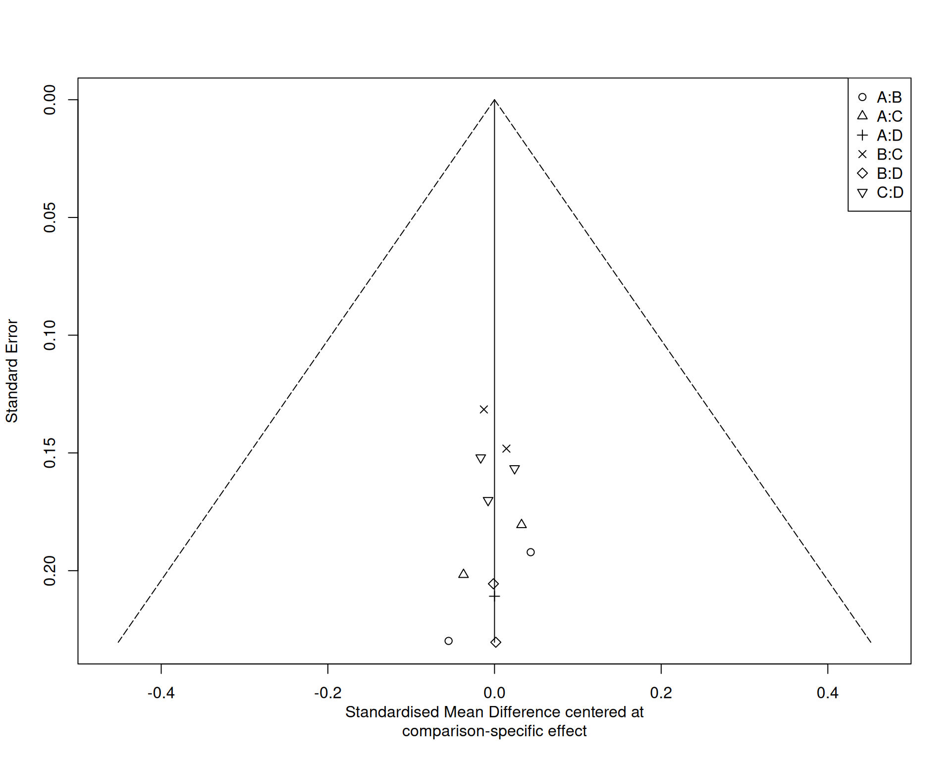
漏斗圖解讀
- 每個比較用不同符號標記
- 對稱性評估需考慮多重比較
- 小型研究效應可能因比較而異
任務九:敏感度分析
模型選擇敏感度
Code
nma_fixed <- netmeta(
  TE = smd,
  seTE = se,
  treat1 = treat1,
  treat2 = treat2,
  studlab = study,
  data = nma_data,
  sm = "SMD",
  reference.group = "A",
  common = TRUE,
  random = FALSE
)

comparison_df <- data.frame(
  Comparison = c("B vs A", "C vs A", "D vs A"),
  Random = round(c(nma_result$TE.random["B", "A"],
                   nma_result$TE.random["C", "A"],
                   nma_result$TE.random["D", "A"]), 3),
  Fixed = round(c(nma_fixed$TE.common["B", "A"],
                  nma_fixed$TE.common["C", "A"],
                  nma_fixed$TE.common["D", "A"]), 3)
)
knitr::kable(comparison_df, caption = "模型比較")| Comparison | Random | Fixed |
|---|---|---|
| B vs A | 0.761 | 0.730 |
| C vs A | 0.993 | 1.003 |
| D vs A | 1.348 | 1.361 |
穩健性判斷
- 排除任一研究後,排名是否改變?
- 固定效應與隨機效應結果是否一致?
- 結論是否穩健?
任務十:學術報告
PRISMA-NMA 報告要素
必要項目
- 網絡幾何圖
- League table
- 一致性評估
進階項目
- 排名(SUCRA/P-score)
- 發表偏誤
- 敏感度分析
結果摘要
Code
# 建立排名摘要
rank_summary <- data.frame(
  Treatment = names(ranking$Pscore.random),
  P_score = round(ranking$Pscore.random, 3)
)
rank_summary <- rank_summary[order(-rank_summary$P_score), ]

summary_df <- data.frame(
  指標 = c("納入研究數", "治療選項數", "總樣本數",
           "最佳治療", "P-score", "I²"),
  數值 = c(nma_result$k,
           nma_result$n,
           sum(nma_data$n1) + sum(nma_data$n2),
           rank_summary$Treatment[1],
           paste0(rank_summary$P_score[1] * 100, "%"),
           paste0(round(nma_result$I2, 1), "%"))
)
knitr::kable(summary_df, caption = "網絡統合分析結果摘要")| 指標 | 數值 |
|---|---|
| 納入研究數 | 12 |
| 治療選項數 | 4 |
| 總樣本數 | 1642 |
| 最佳治療 | A |
| P-score | 100% |
| I² | 0.4% |
檢核清單
準備階段
| 項目 | 完成 |
|---|---|
| 明確定義研究問題 (PICO) | ☐ |
| 事先註冊 (PROSPERO) | ☐ |
| 確認網絡可連通 | ☐ |
分析階段
| 項目 | 完成 |
|---|---|
| 繪製網絡幾何圖 | ☐ |
| 執行網絡統合分析 | ☐ |
| 評估一致性 | ☐ |
| 計算治療排名 | ☐ |
| 敏感度分析 | ☐ |
報告階段
| 項目 | 完成 |
|---|---|
| 遵循 PRISMA-NMA 指引 | ☐ |
| 呈現 League table | ☐ |
| GRADE 評估證據品質 | ☐ |
課程總結
學習重點回顧
- 概念理解:直接證據、間接證據、混合證據
- 網絡幾何:連通性、節點、邊
- 一致性:全域檢定、局部檢定
- 排名:P-score、SUCRA
- 報告:PRISMA-NMA 指引
NMA vs. 傳統統合分析
| 面向 | 傳統統合分析 | 網絡統合分析 |
|---|---|---|
| 比較數 | 2 種治療 | ≥ 3 種治療 |
| 證據類型 | 僅直接 | 直接 + 間接 |
| 排名 | 無 | 有 |
| 一致性 | 不適用 | 需評估 |
延伸學習資源
問答時間
感謝參與!
有任何問題歡迎討論
Network Meta-analysis Course